Central Limit Theorem and Confidence Intervals for Population Proportions

Central Limit Theorem for Sample Proportions

Understanding Sample Proportions

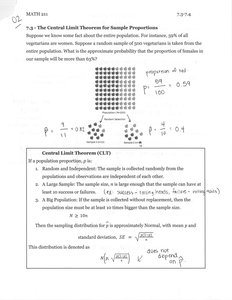
The sample proportion is a statistic that estimates the proportion of a certain characteristic in a population. For example, if 59% of vegetables are tomatoes in a population, the sample proportion is the fraction of tomatoes in a random sample.

• Population proportion (p): The true proportion in the population.

• Sample proportion (\hat{p}): The proportion observed in the sample.

• Random sampling: Ensures that each member of the population has an equal chance of being selected.

Central Limit Theorem (CLT) for Proportions

The Central Limit Theorem states that, under certain conditions, the sampling distribution of the sample proportion \hat{p} will be approximately Normal.

• Conditions:

  • Random and independent sampling

  • Sample size is large enough: both np >= 10 and n(1-p) >= 10

• Mean of sampling distribution: $\mu_{\hat{p}} = p$

• Standard deviation: $\sigma_{\hat{p}} = \sqrt{\frac{p(1-p)}{n}}$

• Normal approximation: $\hat{p} \sim N\left(p, \sqrt{\frac{p(1-p)}{n}}\right)$

Applying the CLT to Real Examples

Checking CLT Conditions

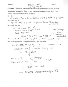
Before applying the CLT, verify that the sample size is large enough for both successes and failures.

• np >= 10: Ensures enough successes in the sample.

• n(1-p) >= 10: Ensures enough failures in the sample.

Example: Proportion of Females in a Group

Suppose p = 0.25 and n = 100. Check if CLT applies:

• np = 100 × 0.25 = 25 > 10

• n(1-p) = 100 × 0.75 = 75 > 10

• CLT applies; the sampling distribution is approximately Normal.

• Mean: $0.25$

• Standard deviation: $\sqrt{\frac{0.25 \times 0.75}{100}} = 0.043$

• Distribution: $N(0.25, 0.043)$

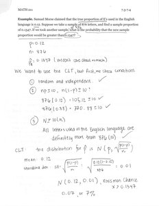
Example: Proportion of 'E's in English Text

Suppose p = 0.12 and n = 876. Check if CLT applies:

• np = 876 × 0.12 = 105 > 10

• n(1-p) = 876 × 0.88 = 772 > 10

• CLT applies; the sampling distribution is approximately Normal.

• Mean: $0.12$

• Standard deviation: $\sqrt{\frac{0.12 \times 0.88}{876}} = 0.01$

• Distribution: $N(0.12, 0.01)$

• 

Estimating Population Proportion with Confidence Intervals

Confidence Intervals for Proportions

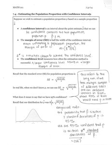
A confidence interval estimates the population proportion based on a sample proportion. It provides a range of plausible values for the true proportion.

• Confidence interval: $\hat{p} \pm z^* \times SE$

• Standard error (SE): $SE = \sqrt{\frac{\hat{p}(1-\hat{p})}{n}}$

• Margin of error (ME): $ME = z^* \times SE$

• z*: Critical value from the Normal distribution for the desired confidence level.

Common Values for Margin of Error

The margin of error depends on the confidence level. Higher confidence levels require larger margins of error.

Confidence Level	Margin of Error
90%	1.65 × SE
95%	1.96 × SE
99%	2.58 × SE

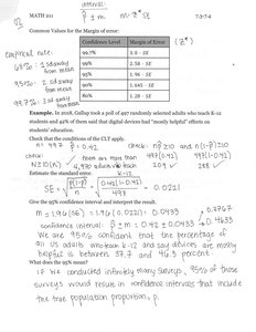
Example: Estimating Proportion of Adults Who Teach K-12

Suppose a poll finds that 27.6% of adults teach K-12. With n = 1000:

• SE: $\sqrt{\frac{0.276 \times 0.724}{1000}} = 0.014$

• 95% CI: $0.276 \pm 1.96 \times 0.014 = (0.249, 0.303)$

• Interpretation: We are 95% confident that the true proportion is between 24.9% and 30.3%.

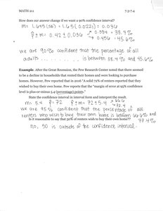
Example: Changing Confidence Level

For a 90% confidence interval, use z* = 1.65:

• CI: $0.276 \pm 1.65 \times 0.014 = (0.254, 0.298)$

• Interpretation: We are 90% confident that the true proportion is between 25.4% and 29.8%.

Summary and Interpretation

Key Points

• The Central Limit Theorem allows us to use Normal models for sample proportions when conditions are met.

• Confidence intervals provide a range of plausible values for the population proportion.

• Margin of error increases with higher confidence levels.

• Interpretation of confidence intervals: "We are X% confident that the true proportion is between A and B."

Additional info: These notes cover material from Chapter 8 (Hypothesis Testing for Population Proportions) and Chapter 9 (Inferring Population Means), specifically focusing on the Central Limit Theorem and confidence intervals for proportions.