6.4 Central Limit Theorem and Normal Probability Distributions: Study Notes

Normal Probability Distributions

The Central Limit Theorem (CLT)

The Central Limit Theorem is a fundamental concept in statistics that allows us to use the normal distribution for the sampling distribution of the sample mean, even when the original population distribution is not normal. This theorem is crucial for many statistical applications, especially when dealing with large samples.

• Definition: The CLT states that for all samples of the same size n with n > 30, the sampling distribution of the sample mean (\bar{x}) can be approximated by a normal distribution with mean \mu and standard deviation \frac{\sigma}{\sqrt{n}}.

• Requirements: The population must be normally distributed or the sample size must be greater than 30.

• Mean of Sample Means: $\mu_{\bar{x}} = \mu$

• Standard Deviation of Sample Means (Standard Error): $\sigma_{\bar{x}} = \frac{\sigma}{\sqrt{n}}$

• Z-score for Sample Mean: $z = \frac{\bar{x} - \mu}{\sigma / \sqrt{n}}$

Note: If the original population is not normally distributed and n ≤ 30, the distribution of \bar{x} cannot be well approximated by a normal distribution. In such cases, nonparametric or bootstrapping methods should be used.

Practical Rules for Applications Involving Sample Means

When applying the CLT in real-world scenarios, it is important to check the requirements and use the correct formulas for individual values and sample means.

• Check Requirements: Confirm that the original population is normal or n > 30.

• Individual Value vs. Sample Mean:

  • For an individual value from a normal population: $z = \frac{x - \mu}{\sigma}$

  • For a sample mean: $z = \frac{\bar{x} - \mu}{\sigma / \sqrt{n}}$

• Notation: The mean of all sample means is \mu_{\bar{x}}, and the standard deviation is \sigma_{\bar{x}} (standard error).

Applications of the Central Limit Theorem

Example: Boeing 737 Airline Seats

This example demonstrates the use of the CLT in evaluating the probability of certain events related to seat design in aircrafts.

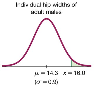
• Scenario: Adult males have hip widths normally distributed with mean 14.3 in. and standard deviation 0.9 in. The seat width is being considered for reduction from 16.6 in. to 16.0 in.

• Part (a): Find the probability that a randomly selected adult male has a hip width greater than 16.0 in.

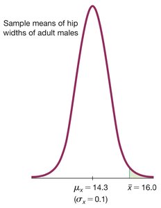
• Part (b): Find the probability that the mean hip width of 126 males is greater than 16.0 in.

• Part (c): Determine which result is more relevant for seat design.

Solution (a): Individual Value

For an individual value, use the z-score formula:

• $z = \frac{x - \mu}{\sigma} = \frac{16.0 - 14.3}{0.9} = 1.89$

• The probability that a randomly selected male has a hip width greater than 16.0 in. is approximately 0.0295 (or 2.95%).

Solution (b): Sample Mean

For the mean of a sample of 126 males, use the CLT:

• $\mu_{\bar{x}} = \mu = 14.3$

• $\sigma_{\bar{x}} = \frac{\sigma}{\sqrt{n}} = \frac{0.9}{\sqrt{126}} \approx 0.1$

• $z = \frac{\bar{x} - \mu_{\bar{x}}}{\sigma_{\bar{x}}} = \frac{16.0 - 14.3}{0.1} = 17.00$

• The probability that the mean hip width of 126 males is greater than 16.0 in. is extremely small (approximately 0.0001).

Interpretation

The result from part (a) is more relevant for seat design, as individual seats are occupied by individual passengers. Although only about 3% of adult males would have hip widths greater than the seat width, this could lead to significant challenges for passengers and flight crew. The reduction of seat width to 16.0 in. does not appear feasible.

Introduction to Hypothesis Testing

The Rare Event Rule for Inferential Statistics

Hypothesis testing involves identifying significant results using probabilities. The rare event rule states that if, under a given assumption, the probability of a particular observed event is very small and the event occurs, we conclude that the assumption is probably not correct.

Example: Body Temperatures

This example illustrates hypothesis testing using the CLT and the rare event rule.

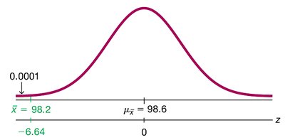
• Scenario: Assume the population mean body temperature is 98.6°F with a standard deviation of 0.62°F. A sample of 106 subjects yields a mean of 98.2°F.

• Question: If the mean is really 98.6°F, what is the probability of getting a sample mean of 98.2°F or lower?

Solution

• $\mu_{\bar{x}} = \mu = 98.6$

• $\sigma_{\bar{x}} = \frac{\sigma}{\sqrt{n}} = \frac{0.62}{\sqrt{106}} \approx 0.0602$

• $z = \frac{\bar{x} - \mu_{\bar{x}}}{\sigma_{\bar{x}}} = \frac{98.2 - 98.6}{0.0602} = -6.64$

• The probability of obtaining a sample mean of 98.2°F or lower is approximately 0.0001.

Interpretation

Since the probability is extremely low, it is more reasonable to conclude that the population mean is lower than 98.6°F. The true mean body temperature appears to be closer to 98.2°F.

Summary Table: Central Limit Theorem Parameters

Parameter	Symbol	Formula	Description
Population Mean	\mu	—	Mean of the original population
Sample Mean	\bar{x}	—	Mean of a sample of size n
Standard Deviation of Population	\sigma	—	Standard deviation of the original population
Standard Error (Sample Means)	\sigma_{\bar{x}}	$\frac{\sigma}{\sqrt{n}}$	Standard deviation of sample means
Z-score (Individual Value)	z	$\frac{x - \mu}{\sigma}$	Standardized score for individual value
Z-score (Sample Mean)	z	$\frac{\bar{x} - \mu}{\sigma / \sqrt{n}}$	Standardized score for sample mean