Chapter 14: Sampling Distribution Models – Central Limit Theorem and Applications

Sampling Distribution Models

Introduction to Sampling Distributions

In statistics, we often estimate unknown population parameters (such as the mean, proportion, or standard deviation) using sample statistics. Because these statistics vary from sample to sample, understanding their distribution is crucial for making reliable inferences about the population.

• Parameter: A numerical characteristic of a population (e.g., population mean μ, population proportion p).

• Statistic: A numerical characteristic calculated from a sample (e.g., sample mean \bar{x}, sample proportion \hat{p}).

• Sampling Distribution: The probability distribution of a given statistic based on a random sample.

Sampling distributions allow us to judge the reliability of a sample statistic as an estimator of the corresponding population parameter.

Constructing a Sampling Distribution

To visualize a sampling distribution, imagine repeatedly drawing random samples of size n from a population and calculating a statistic (such as the mean) for each sample. Plotting these statistics forms the sampling distribution.

• The distribution of the sample means (or proportions, etc.) is called the sampling distribution of that statistic.

• The shape of the sampling distribution depends on the sample size and the population distribution.

The Central Limit Theorem (CLT)

Statement and Importance

The Central Limit Theorem (CLT) is a fundamental result in statistics. It states that, for a sufficiently large sample size, the sampling distribution of the sample mean (or proportion) will be approximately normal, regardless of the shape of the population distribution.

• Requirements: Observations must be independent and randomly sampled.

• Sample Size: The larger the sample size, the closer the sampling distribution is to normality. For most populations, n ≥ 30 is often sufficient; for highly skewed populations, larger samples may be needed.

The CLT enables us to use the normal model for inference about means and proportions, even when the population is not normal.

Properties of the Sampling Distribution of the Mean

• Mean: The mean of the sampling distribution of the sample mean is equal to the population mean: $\mu_{\bar{y}} = \mu$

• Standard Deviation (Standard Error): The standard deviation of the sampling distribution of the sample mean is: $\sigma_{\bar{y}} = \frac{\sigma}{\sqrt{n}}$

• As n increases, the sampling distribution becomes more concentrated around the population mean, and its standard deviation decreases.

Illustrative Example: Supermarket Checkout Times

Suppose we have a population of 500 supermarket checkout times. By drawing repeated samples of size n = 5 and n = 25, and calculating the sample means, we observe:

• The mean of the sample means is close to the population mean.

• The standard deviation of the sample means decreases as n increases.

• The sampling distribution becomes more symmetric and normal as n increases, even if the population is skewed.

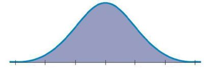
Visual Representation of Sampling Distributions

The following image illustrates the normal shape of a sampling distribution as predicted by the Central Limit Theorem:

Application: Probability Calculations Using the CLT

Example: Rice Krispies Bar Weights

Suppose the weight of a rice-krispie bar is normally distributed with mean 22.2g and standard deviation 0.40g. We can use the CLT to answer questions about individual bars and the mean weight in a box of 24 bars:

• Probability for One Bar: Use the population mean and standard deviation.

• Probability for the Mean of 24 Bars: Use the sampling distribution of the mean, with standard error $\sigma_{\bar{y}} = \frac{0.40}{\sqrt{24}} \approx 0.08165$.

The probability that the mean weight in a box of 24 bars is below the stated amount is much smaller than for a single bar, reflecting the reduced variability of the sample mean.

Sampling Distribution of Sample Proportions

CLT for Proportions

The Central Limit Theorem also applies to sample proportions. If we repeatedly sample and calculate the proportion of successes, the sampling distribution of the sample proportion $\hat{p}$ will be approximately normal for large enough samples.

• Mean: $\mu_{\hat{p}} = p$

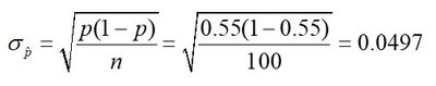
• Standard Deviation (Standard Error): $\sigma_{\hat{p}} = \sqrt{\frac{p(1-p)}{n}}$

For example, if the true proportion of brown-haired people is 0.55 and we sample 100 people, the standard error is:

Assumptions and Conditions for the CLT

• Independence Assumption: Sampled values must be independent.

• Randomization Condition: The sample should be a simple random sample.

• 10% Condition: If sampling without replacement, sample size should be less than 10% of the population.

• Success/Failure Condition: Both $np$ and $n(1-p)$ should be at least 10.

Common Pitfalls and Final Notes

• Do not confuse the sampling distribution (distribution of a statistic over all possible samples) with the distribution of the sample (distribution of observed values in one sample).

• The CLT allows us to use the normal model for inference about means and proportions, provided assumptions are met.

• Sampling distributions arise because samples vary; the CLT saves us from simulating distributions for means and proportions.

Summary Table: Key Properties of Sampling Distributions

Statistic	Mean of Sampling Distribution	Standard Deviation (Standard Error)	CLT Conditions
Sample Mean ($\bar{y}$)	$\mu_{\bar{y}} = \mu$	$\sigma_{\bar{y}} = \frac{\sigma}{\sqrt{n}}$	Independence, Large Enough $n$
Sample Proportion ($\hat{p}$)	$\mu_{\hat{p}} = p$	$\sigma_{\hat{p}} = \sqrt{\frac{p(1-p)}{n}}$	Independence, $np \geq 10$, $n(1-p) \geq 10$