Chapter 14: Sampling Distribution Models – Study Notes

Sampling Distribution Models

Introduction to Sampling Distributions

In statistics, we often estimate unknown population parameters (such as the mean, proportion, or standard deviation) using sample statistics. Because these statistics vary from sample to sample, understanding their distribution is crucial for making reliable inferences about the population.

• Parameter: A numerical characteristic of a population (e.g., population mean μ, population proportion p).

• Statistic: A numerical characteristic calculated from a sample (e.g., sample mean \bar{x}, sample proportion \hat{p}).

• Point Estimate: A sample statistic used to estimate a population parameter.

The sampling distribution of a statistic is the probability distribution of that statistic, considering all possible random samples of a fixed size from the population.

Constructing a Sampling Distribution

To visualize a sampling distribution, imagine repeatedly drawing random samples of size n from a population, calculating the statistic (e.g., mean) for each sample, and plotting these values in a histogram. The resulting distribution is the sampling distribution of the statistic.

• The sampling distribution helps us judge the reliability of a sample statistic as an estimator of the population parameter.

• In practice, we use mathematical theory or computer simulation to approximate the sampling distribution.

Example: Supermarket Checkout Times

Suppose we have a population of 500 supermarket checkout times. We want to estimate the population mean μ. By simulating 100 random samples of size n = 5 and calculating their means, we observe:

• The sample means are much closer to each other than the individual values in each sample.

• The histogram of sample means is more symmetric and normal than the population distribution, though still right-skewed for small n.

Impact of Sample Size (n)

As the sample size increases, the sampling distribution of the sample mean becomes more symmetric and approaches a normal distribution, even if the population is skewed. The spread (standard deviation) of the sample means decreases as n increases.

Variable	N	Mean	StDev
Population (Time)	500	50.12	49.06
Sample Means (n = 5)	100	48.83	23.60
Sample Means (n = 25)	100	50.16	9.85

Key Observations:

• The mean of the sample means is close to the population mean.

• The standard deviation of the sample means decreases as n increases.

J

The Central Limit Theorem (CLT)

Statement and Importance

The Central Limit Theorem (CLT) is a fundamental result in statistics. It states that, for a sufficiently large sample size, the sampling distribution of the sample mean will be approximately normal, regardless of the shape of the population distribution, provided the observations are independent and randomly sampled.

• The mean of the sampling distribution is the population mean μ.

• The standard deviation of the sampling distribution (standard error) is $\sigma_{\bar{y}} = \frac{\sigma}{\sqrt{n}}$

As n increases, the normal model becomes a better approximation for the sampling distribution of the mean.

Properties of the Sampling Distribution of the Mean

• Mean: $\mu_{\bar{y}} = \mu$

• Standard Deviation (Standard Error): $\sigma_{\bar{y}} = \frac{\sigma}{\sqrt{n}}$

These properties are supported by both simulation and theory.

Sampling Error and Variability

The variability of sample means about the true population mean is called the sampling error or sampling variability. This variability decreases as the sample size increases.

Assumptions and Conditions for the CLT

• Independence Assumption: Sampled values must be independent.

• Sample Size Assumption: The sample size n must be large enough (often n ≥ 30 is sufficient, but more may be needed for highly skewed populations).

Application Example: Rice Krispies Bars

Suppose the weight of a rice-crispie bar is normally distributed with mean 22.2g and standard deviation 0.40g. For boxes of 24 bars:

• Probability a single bar is below 22g: Use population mean and standard deviation.

• Probability the mean weight in a box of 24 bars is below 22g: Use the CLT and the sampling distribution of the mean.

Sampling Distribution of Sample Proportions

The Central Limit Theorem for Proportions

The CLT also applies to sample proportions. If we repeatedly sample and calculate the proportion of successes, the sampling distribution of the sample proportion \hat{p} will be approximately normal for large enough n.

• Mean: $\mu_{\hat{p}} = p$

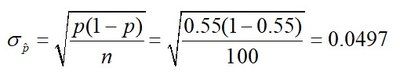
• Standard Deviation (Standard Error): $\sigma_{\hat{p}} = \sqrt{\frac{p(1-p)}{n}}$

Simulation Example: Brown Hair Proportion

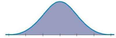
If we sample 100 people 1000 times and record the proportion with brown hair (true population proportion = 0.55), the histogram of sample proportions will be approximately normal, centered at 0.55, with standard deviation close to the theoretical value.

Assumptions and Conditions for Proportions

• Independence Assumption: Sampled values must be independent.

• Sample Size Assumption: Sample size must be large enough.

• Randomization Condition: The sample should be a simple random sample.

• 10% Condition: If sampling without replacement, n should be no more than 10% of the population.

• Success/Failure Condition: Both np and n(1-p) should be at least 10.

Real World vs. Model World

It is important to distinguish between the distribution of the sample (real world) and the sampling distribution of the statistic (model world). The CLT allows us to use the normal model for the sampling distribution, but not for the distribution of the sample itself.

Summary Table: Sampling Distribution Properties

Statistic	Mean	Standard Deviation
Sample Mean (\bar{y})	$\mu$	$\frac{\sigma}{\sqrt{n}}$
Sample Proportion (\hat{p})	$p$	$\sqrt{\frac{p(1-p)}{n}}$

Common Pitfalls

• Do not confuse the sampling distribution with the distribution of the sample.

• Ensure independence of observations; the CLT does not apply if data are not independent.

• For highly skewed populations, larger sample sizes are needed for the CLT to hold.

What Have We Learned?

• The Central Limit Theorem allows us to model the sampling distribution of the sample mean and proportion as normal for large enough samples.

• The mean of the sampling distribution equals the population parameter, and the standard deviation decreases with increasing sample size.

• Always check the necessary assumptions and conditions before applying the CLT.