Chapter 18: Inferences About Means – The t-Distribution and Small Sample Inference

Inferences About Means

Introduction to Inference for Means

Statistical inference about population means is a fundamental topic in statistics. When the population standard deviation (σ) is unknown and the sample size is small, we must use special methods to account for extra uncertainty. This chapter focuses on the use of the Student's t-distribution for constructing confidence intervals and hypothesis tests about means under these conditions.

The Central Limit Theorem (CLT) Revisited

Sampling Distribution of the Mean

• Central Limit Theorem (CLT): For sufficiently large sample sizes, the sampling distribution of the sample mean is approximately normal, regardless of the population's distribution.

• Mean and Standard Deviation: The sampling distribution has mean equal to the population mean (μ) and standard deviation equal to the population standard deviation divided by the square root of the sample size:

$\text{Mean of } \bar{y} = \mu \\ \text{Standard deviation of } \bar{y} = \frac{\sigma}{\sqrt{n}}$

• When σ is unknown, we estimate it with the sample standard deviation (s), leading to the standard error:

$SE(\bar{y}) = \frac{s}{\sqrt{n}}$

Student's t-Distribution

Origin and Properties

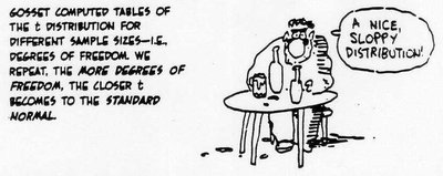
• William S. Gosset (pseudonym "Student") developed the t-distribution while working at Guinness Brewery.

• The t-distribution is used when the population standard deviation is unknown and the sample size is small.

• The t-distribution forms a family of distributions indexed by degrees of freedom (df), typically df = n - 1.

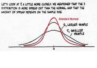
• Compared to the standard normal (z) distribution, the t-distribution is flatter and has heavier tails, reflecting greater uncertainty.

• As the sample size increases (df increases), the t-distribution approaches the standard normal distribution.

Key Characteristics of the t-Distribution

• Unimodal and symmetric about zero.

• Mean of zero.

• Heavier tails than the normal distribution (more probability in the tails).

• Shape depends on degrees of freedom (df = n - 1).

• As df → ∞, t-distribution becomes the standard normal distribution.

Using the t-Distribution for Inference

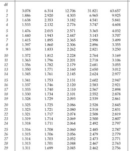
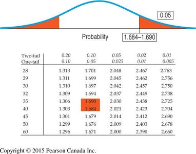
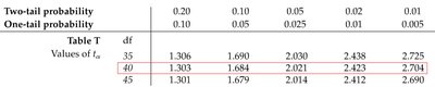
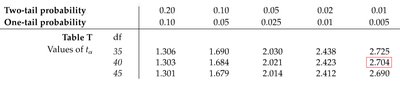
t-Distribution Tables and Critical Values

• Tables provide critical values for selected confidence levels and degrees of freedom.

• For large df, t-values approach z-values.

• Common tail probabilities: 0.10, 0.05, 0.025, 0.01, 0.005.

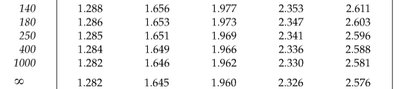
• For degrees of freedom not listed, approximate by using the next lower df or use statistical software.

Degrees of Freedom and Sample Standard Deviation

• Sample standard deviation is calculated using n - 1 in the denominator to correct for bias when estimating from the sample mean:

$s = \sqrt{\frac{\sum (y_i - \bar{y})^2}{n-1}}$

• This adjustment is called the degrees of freedom correction.

Confidence Intervals for the Mean (t-Interval)

Constructing a t-Interval

When the sample size is small (n < 60) and σ is unknown, the confidence interval for the population mean is:

$\bar{y} \pm t_{\alpha/2, df} \cdot SE(\bar{y})$

where $SE(\bar{y}) = \frac{s}{\sqrt{n}}$ and $t_{\alpha/2, df}$ is the critical value from the t-distribution with df = n - 1.

• t-intervals are wider than z-intervals, reflecting extra uncertainty from estimating σ.

One-Sample t-Test for the Mean

Hypothesis Testing Procedure

• Used when testing hypotheses about a population mean with unknown σ and small n.

• Test statistic:

$t = \frac{\bar{y} - \mu_0}{s/\sqrt{n}}$

• Compare the calculated t to the critical value from the t-table, or use the p-value approach.

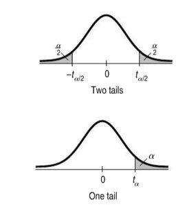
• Types of tests: lower-tailed, upper-tailed, and two-tailed.

Assumptions and Conditions for t-Methods

• Independence Assumption: Data values must be independent.

• Randomization Condition: Data should come from a random sample or randomized experiment.

• 10% Condition: Sample size should be less than 10% of the population when sampling without replacement.

• Normal Population Assumption: The population should be approximately normal, or the sample size should be large enough for the CLT to apply.

• Nearly Normal Condition: For small samples, check for unimodality and symmetry using histograms, boxplots, or normal probability plots.

Examples

Example 1: Humerus Bones

• Archaeologists test whether unearthed bones belong to species A (mean ratio = 8.5).

• Sample: n = 41, mean = 9.258, s = 1.204, SE = 0.188.

• Hypotheses: $H_0: \mu = 8.5$, $H_a: \mu \neq 8.5$

• Test statistic: $t = \frac{9.258 - 8.5}{0.188} = 4.031$

• p-value < 0.01, so reject $H_0$; bones are not from species A.

• 99% CI: $9.258 \pm 2.704 \times 0.188 = [8.75, 9.77]$

• Assumptions checked: Histogram and boxplot show unimodal, symmetric data with two outliers; normality test p-value > 0.05.

Example 2: Apple Juice Fill

• Quality control manager tests if bottles are under-filled (target = 64.05 oz).

• Sample: n = 22, mean = 64.0073, s = 0.0446, SE = 0.0095.

• Hypotheses: $H_0: \mu = 64.05$, $H_a: \mu < 64.05$

• Test statistic: $t = \frac{64.0073 - 64.05}{0.0095} = -4.49$

• p-value < 0.01, so reject $H_0$; mean fill is lower than target.

• 99% upper bound: 64.0312 oz.

• Assumptions: Boxplot is symmetric, data are normal, random sample, n < 10% of population.

Sample Size Determination

Calculating Required Sample Size

• To estimate the mean within a margin of error (ME) at a given confidence level, solve:

$n = \left( \frac{z^* s}{ME} \right)^2$

• Use s from a pilot study if σ is unknown.

• For the apple juice example, to estimate the mean within 0.01 oz at 99% confidence (z* = 2.576, s = 0.0446):

$n = \left( \frac{2.576 \times 0.0446}{0.01} \right)^2 \approx 132$

Common Pitfalls and Best Practices

• Do not confuse means and proportions.

• Check for multimodality and skewness; t-methods are robust to mild deviations from normality, but not to severe ones.

• Beware of outliers and bias; always report on outliers and ensure random sampling.

• Interpret confidence intervals correctly: they refer to the population mean, not individual values.

• Choose the alternative hypothesis before seeing the data.

Summary of Key Formulas

• Standard Error: $SE(\bar{y}) = \frac{s}{\sqrt{n}}$

• Confidence Interval: $\bar{y} \pm t_{\alpha/2, df} \cdot SE(\bar{y})$

• t-Test Statistic: $t = \frac{\bar{y} - \mu_0}{s/\sqrt{n}}$

• Sample Size: $n = \left( \frac{z^* s}{ME} \right)^2$

What Have We Learned?

• How to use the t-distribution for inference about means when σ is unknown and n is small.

• How to construct confidence intervals and perform hypothesis tests using the t-distribution.

• The importance of checking assumptions and conditions before applying t-methods.

• How to determine the required sample size for a desired margin of error.