Chapter 23: Inferences for Regression – Study Notes

Inferences for Regression

Introduction to Regression Analysis

Regression analysis is a statistical method used to model and analyze the relationship between a dependent (response) variable and one or more independent (predictor) variables. The goal is to predict or explain the dependent variable using the independent variable(s).

• Dependent variable (y): The outcome or variable to be predicted.

• Independent variable (x): The variable used to predict y.

• The equation for the line of best fit (simple linear regression): $\hat{y} = b_0 + b_1 x$

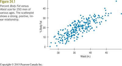
Example: Predicting percent body fat from waist size in men.

The Population Regression Model

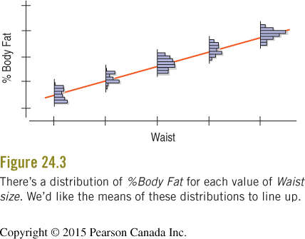
We use regression to make inferences about the population, not just the sample. The idealized regression line for the population is written as:

• $\mu_y = \beta_0 + \beta_1 x$

• For individual data points, we include random error: $y = \beta_0 + \beta_1 x + \varepsilon$

• Where $\varepsilon$ is the residual error, assumed to be random and normally distributed.

Key Terms:

• Intercept ($\beta_0$): Expected value of y when x = 0.

• Slope ($\beta_1$): Expected change in y for a one-unit increase in x.

• Residual ($\varepsilon$): The difference between observed and predicted y.

Assumptions and Conditions for Regression Inference

1. Linearity Assumption

The relationship between x and y must be linear. This is checked using a scatterplot of the data (Straight Enough Condition).

• If the scatterplot is not linear, consider transforming the data.

2. Independence Assumption

The observations must be independent. This is often ensured by random sampling (Randomization Condition). Independence can also be checked by plotting residuals versus the x-variable; the residuals should appear randomly scattered.

3. Equal Variance Assumption (Homoscedasticity)

The spread of the residuals should be roughly constant for all values of x (Does the Plot Thicken? Condition). This is checked using a residuals vs fits plot.

• If the spread increases or decreases with x, the assumption is violated.

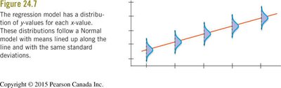
4. Normal Population Assumption

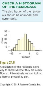
The residuals should be nearly normally distributed (Nearly Normal Condition). This is checked using a histogram or a normal probability plot of the residuals. Outliers should also be checked.

Summary of Assumptions

• Linearity: Relationship between x and y is linear.

• Independence: Observations are independent.

• Equal Variance: Residuals have constant variance.

• Normality: Residuals are normally distributed.

Order of Conducting a Simple Regression Analysis

1. Check linearity with a scatterplot.

2. Fit the regression model and examine residuals vs fits plot for patterns.

3. Check the histogram and normal probability plot of residuals for normality.

4. If data are time series, plot residuals vs time to check for independence.

Intuition About Regression Inference

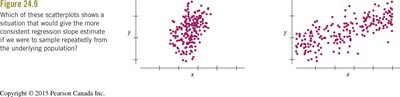
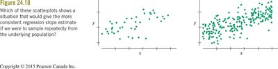
Factors Affecting the Standard Error of the Slope

• Spread around the line (se): Less scatter means more consistent slope estimates.

• Spread of x values (sx): Greater spread in x gives more stable regression estimates.

• Sample size (n): Larger sample size gives more consistent estimates.

Standard Error of the Slope

The standard error of the regression slope is calculated as:

$SE(b_1) = \frac{s_e}{s_x \sqrt{n-1}}$

• $s_e$ = residual standard deviation

• $s_x$ = standard deviation of x-values

• $n$ = sample size

Inference for Regression Slope

Hypothesis Test for Slope

• Null hypothesis: $H_0: \beta_1 = 0$ (no relationship between x and y)

• Alternative hypothesis: $H_A: \beta_1 \neq 0$ (x and y are related)

• Test statistic: $t = \frac{b_1 - 0}{SE(b_1)}$ with $n-2$ degrees of freedom

• Confidence interval for slope: $b_1 \pm t_{\alpha/2, n-2} SE(b_1)$

Example: Testing the Relationship Between % Body Fat and Waist Size

Term	Coef	SE Coef	T-Value	P-Value
Constant	-62.6	10.2	-6.16	0.000
Waist	2.222	0.273	8.14	0.000

• Test statistic: $t = \frac{2.222}{0.273} = 8.14$

• P-value < 0.05, so we reject $H_0$ and conclude a significant linear relationship exists.

Confidence Interval for the Slope

For 95% confidence and 18 degrees of freedom:

$2.222 \pm 2.10092 \times 0.273 = [1.648, 2.796]$

Interpretation: For every 1 inch increase in waist size, percent body fat increases by between 1.648% and 2.796%.

Estimation and Prediction Using the Regression Model

Confidence Interval for Mean Response

To estimate the mean value of y for a given x ($x_0$):

$\mu_{y_0} = b_0 + b_1 x_0 \pm t_{\alpha/2, n-2} \cdot SE_{\mu_{y_0}}$

Where $SE_{\mu_{y_0}}$ is the standard error for the mean response at $x_0$.

Prediction Interval for a New Observation

To predict the value of y for a new individual at $x_{new}$:

$Y_{new} = b_0 + b_1 x_{new} \pm t_{\alpha/2, n-2} \cdot SE_{pred}$

Where $SE_{pred}$ includes an extra term for the variability of individual observations.

Comparison of Intervals

• Confidence Interval (CI): For the mean response at a given x; narrower interval.

• Prediction Interval (PI): For a single new observation at a given x; wider interval due to extra uncertainty.

Common Pitfalls in Regression Inference

• Do not fit a linear model to non-linear data.

• Check for non-constant variance (plot thickening).

• Be cautious with extrapolation (predicting outside the range of data).

• Watch for outliers and high-influence points.

• Ensure residuals are nearly normal.

• Use two-tailed tests unless a one-tailed test is justified.

Summary of Key Skills

• Check all regression assumptions before making inferences.

• Interpret regression output, including slope, intercept, standard errors, t-values, and p-values.

• Construct and interpret confidence and prediction intervals.

• Understand the difference between inference for the mean response and for individual predictions.