Chapter 24: Analysis of Variance (ANOVA) – Study Notes

Analysis of Variance (ANOVA)

Introduction to ANOVA

Analysis of Variance (ANOVA) is a statistical method used to test whether the means of three or more groups are equal. It generalizes the two-sample t-test to situations involving more than two groups, allowing for the comparison of multiple treatment means simultaneously.

• Purpose: To determine if observed differences among sample means are statistically significant or could have occurred by random chance.

• Null Hypothesis (H0): All group means are equal.

• Alternative Hypothesis (HA): At least one group mean is different.

Visualizing Group Means

Boxplots are commonly used to visually compare the means and spreads of several groups. The clarity of differences among means depends on the relative size of the variation within groups compared to the differences between group means.

• Large within-group variation can obscure differences between group means.

• Small within-group variation makes differences between group means more apparent.

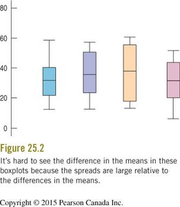
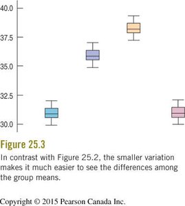
Example: In the first figure, the means are the same as in the second, but the larger spread within groups makes it difficult to distinguish differences in means. In the second figure, smaller within-group variation makes the differences among means stand out.

Concept of Variance in ANOVA

ANOVA compares two sources of variance:

• Between-group variance (MST): Measures how much the group means differ from the overall grand mean.

• Within-group variance (MSE): Measures the variability of observations within each group around their respective group means.

The F-statistic is the ratio of these two variances:

$F = \frac{\text{variation between groups}}{\text{variation within groups}} = \frac{MST}{MSE}$

• If F is large, it suggests significant differences between group means.

• If F is close to 1, it suggests no significant difference between group means.

Calculating Variances and Sums of Squares

• Sum of Squares for Treatments (SST): $SST = \sum_j n_j (\bar{y}_j - \bar{y})^2$

• Sum of Squares for Error (SSE): $SSE = \sum_{i,j} (y_{ij} - \bar{y}_j)^2$

• Total Sum of Squares (SSTotal): $SSTotal = SST + SSE$

• Mean Square for Treatments (MST): $MST = \frac{SST}{k-1}$

• Mean Square Error (MSE): $MSE = \frac{SSE}{N-k}$

Where k is the number of groups, N is the total number of observations, $\bar{y}_j$ is the mean of group j, and $\bar{y}$ is the grand mean.

The F-Distribution and ANOVA Table

The F-statistic follows an F-distribution with degrees of freedom (df) for the numerator (k-1) and denominator (N-k). The results are typically summarized in an ANOVA table:

Source of Variation	Degrees of Freedom	Sum of Squares	Mean Squares	F-statistic	P-value
Treatment (Between)	k-1	SST	MST	F	P
Error (Within)	N-k	SSE	MSE
Total	N-1	SSTotal

The P-value is obtained by comparing the F-statistic to the F-distribution. If the P-value is less than the significance level (e.g., 0.05), we reject the null hypothesis.

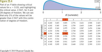
Example: The F-table provides critical values for different combinations of degrees of freedom and significance levels.

Example: Analgesics Experiment

A pharmaceutical company tested three formulations of a pain relief medication on 12 volunteers, with 4 subjects per formulation. The pain level was measured 30 minutes after taking the medication.

• Means: A = 3.25, B = 7.25, C = 6.00, Grand Mean = 5.50

• ANOVA Results: F = 20.10, P-value = 0.000 (significant)

• Conclusion: At least one drug formulation has a different mean pain level.

Assumptions and Conditions for ANOVA

Before interpreting ANOVA results, check the following assumptions:

• Independence: Groups and observations within groups must be independent. Check randomization in study design.

• Equal Variance (Homogeneity): Variances of groups should be similar. Use side-by-side boxplots and residual plots to assess.

• Normality: The residuals should be approximately normally distributed. Check with histograms or normal probability plots.

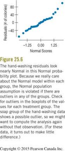
Example: The normal probability plot shows residuals are reasonably normal, supporting the normality assumption.

Multiple Comparisons and Tukey's Test

If the ANOVA F-test is significant, further analysis is needed to determine which means differ. Multiple comparison procedures, such as Tukey's test, control the overall Type I error rate when making several pairwise comparisons.

• Tukey's Test: Compares all possible pairs of group means using confidence intervals.

• Interpretation:

  • If the confidence interval for the difference contains 0, the means are not significantly different.

  • If the interval is entirely positive or negative, one mean is significantly greater or less than the other.

• Number of comparisons: $c = \frac{k(k-1)}{2}$

What Can Go Wrong?

• Outliers: Can distort the F-test and conclusions.

• Unequal variances: May require transformation of the response variable.

• Multiple comparisons: Increases risk of Type I error; always use a multiple comparisons method.

• Observational studies: Be cautious about inferring causality.

Summary of Key Points

• ANOVA tests for equality of means across multiple groups using the F-statistic.

• Check assumptions of independence, equal variance, and normality before interpreting results.

• Use multiple comparison procedures (e.g., Tukey's test) to identify which means differ after a significant ANOVA result.

• Interpret ANOVA tables and understand the roles of MST, MSE, and the F-statistic.