Chapter 3: Describing, Exploring, and Comparing Data – Study Notes

Describing, Exploring, and Comparing Data

Overview

This chapter focuses on methods for summarizing and comparing data sets. The main topics include measures of center, measures of variation, and measures of relative standing, which are fundamental for understanding and interpreting statistical data.

Measures of Center

Definition and Importance

Measures of center are values that represent the middle or central point of a data set. They help summarize a data set with a single value, making it easier to interpret and compare.

• Mean (Arithmetic Mean): The sum of all data values divided by the number of values. It is sensitive to outliers and uses every data value.

• Median: The middle value when data is ordered. It is resistant to outliers and does not use every data value directly.

• Mode: The value(s) that occur most frequently. Can be used with qualitative data and may have no mode, one mode, or multiple modes.

• Midrange: The value midway between the maximum and minimum values. It is not resistant to outliers and is rarely used in practice.

Mean (Arithmetic Mean)

The mean is calculated as follows:

• Sample Mean: $x\ =\ \frac{\sum x}{n}$

• Population Mean: $\mu\ =\ \frac{\sum x}{N}$

Properties:

• Sample means vary less than other measures of center.

• Mean is not resistant to outliers.

Median

The median is found by sorting the data and:

• If odd number of values: Median is the middle value.

• If even number of values: Median is the mean of the two middle values.

Properties:

• Median is resistant to outliers.

• Median does not use every data value directly.

Mode

The mode is the value(s) with the highest frequency. Data sets can be:

• Bimodal: Two modes

• Multimodal: More than two modes

• No mode: No repeated values

Midrange

The midrange is calculated as:

• $\text{Midrange}\ =\ \frac{\text{maximum data value}\ +\ \text{minimum data value}}{2}$

Properties:

• Very sensitive to extremes; not resistant.

• Easy to compute.

Round-Off Rules

• Mean, median, midrange: Carry one more decimal place than original data.

• Mode: Leave as is, no rounding.

Critical Thinking

Always consider whether measures of center are meaningful for the data type and the sampling method used.

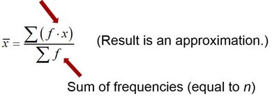
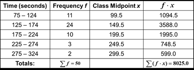
Mean from a Frequency Distribution

When data is summarized in a frequency distribution, the mean is approximated by:

• $\bar{x}\ =\ \frac{\sum (f \cdot x)}{\sum f}$

Weighted Mean

When data values have different weights:

• $\bar{x}\ =\ \frac{\sum (w \cdot x)}{\sum w}$

Measures of Variation

Definition and Importance

Measures of variation describe how spread out the data values are. They are crucial for understanding the reliability and consistency of data.

• Range: Difference between maximum and minimum values.

• Standard Deviation: Measures average deviation from the mean.

• Variance: Square of the standard deviation.

Range

Calculated as:

• $\text{Range}\ =\ \text{maximum data value}\ -\ \text{minimum data value}$

Properties:

• Very sensitive to extremes; not resistant.

• Does not reflect variation among all values.

Standard Deviation

Standard deviation quantifies the spread of data values around the mean.

• Sample Standard Deviation: $s\ =\ \sqrt{\frac{\sum (x - \bar{x})^2}{n - 1}}$

• Population Standard Deviation: $\sigma\ =\ \sqrt{\frac{\sum (x - \mu)^2}{N}}$

Properties:

• Never negative; zero if all values are identical.

• Units are same as original data.

• Sample standard deviation is a biased estimator of population standard deviation.

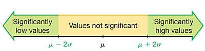
Range Rule of Thumb

Most values lie within 2 standard deviations of the mean. Significant values are those outside this range.

Estimating Standard Deviation

• $s \approx \frac{\text{range}}{4}$

Variance

Variance is the square of the standard deviation.

• Sample Variance: $s^2$

• Population Variance: $\sigma^2$

Properties:

• Units are squares of original units.

• Not resistant to outliers.

• Sample variance is an unbiased estimator of population variance.

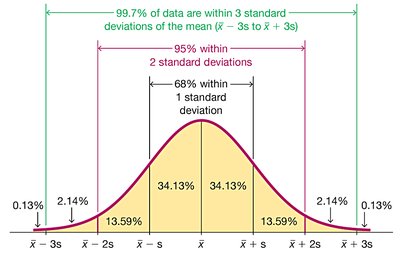
Empirical Rule

For bell-shaped distributions:

• 68% within 1 standard deviation

• 95% within 2 standard deviations

• 99.7% within 3 standard deviations

Chebyshev’s Theorem

For any data set, at least $1 - \frac{1}{k^2}$ of values lie within k standard deviations of the mean (k > 1).

Coefficient of Variation

Expresses standard deviation relative to the mean as a percentage:

• Sample: $CV = \frac{s}{\bar{x}} \times 100$

• Population: $CV = \frac{\sigma}{\mu} \times 100$

Measures of Relative Standing and Boxplots

Definition and Importance

Measures of relative standing indicate the position of a data value within a data set. Common measures include z scores, percentiles, and quartiles. Boxplots visually summarize these measures.

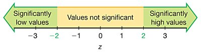
z Scores

A z score shows how many standard deviations a value is from the mean:

• Sample: $z = \frac{x - \bar{x}}{s}$

• Population: $z = \frac{x - \mu}{\sigma}$

Properties:

• z scores have no units.

• z ≤ -2: Significantly low; z ≥ 2: Significantly high.

• Negative z: Value below mean.

Percentiles

Percentiles divide data into 100 groups, each with about 1% of values. To find the percentile of a value:

• Percentile of x = $\frac{\text{number of values less than } x}{\text{total number of values}} \times 100$

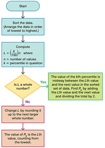
Converting a Percentile to a Data Value

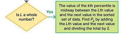
To find the kth percentile:

• Compute locator: $L = \frac{k}{100} \times n$

• If L is a whole number, the percentile is midway between the Lth and (L+1)th values.

• If L is not a whole number, round up and use the Lth value.

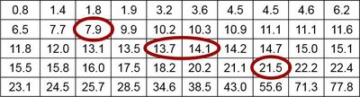
Quartiles

Quartiles divide data into four groups:

• Q1: First quartile (25th percentile)

• Q2: Second quartile (50th percentile, median)

• Q3: Third quartile (75th percentile)

Statistics defined using quartiles:

• Interquartile Range (IQR): $Q_3 - Q_1$

• Semi-interquartile Range: $\frac{Q_3 - Q_1}{2}$

• Midquartile Range: $\frac{Q_1 + Q_3}{2}$

• 10-90 Quartile Range: $P_{90} - P_{10}$

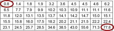
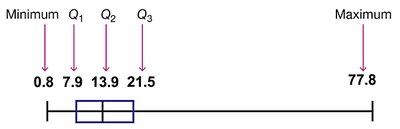
5-Number Summary

The 5-number summary consists of:

• Minimum

• Q1

• Median (Q2)

• Q3

• Maximum

Boxplot (Box-and-Whisker Diagram)

A boxplot is a graphical representation of the 5-number summary. It consists of a box from Q1 to Q3, a line at the median, and whiskers extending to the minimum and maximum values.

Skewness

A boxplot can help identify skewness. A distribution is skewed if it is not symmetric and extends more to one side.

Identifying Outliers for Modified Boxplots

Outliers are values that fall outside the range:

• Above Q3 by more than 1.5 × IQR

• Below Q1 by more than 1.5 × IQR

Modified boxplots mark outliers with special symbols and extend whiskers only to the most extreme non-outlier values.