Chapter 3: Numerically Summarizing Data – Measures of Central Tendency, Dispersion, and Position

Measures of Central Tendency

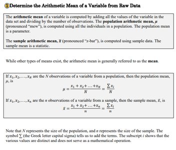
Arithmetic Mean

The arithmetic mean is a measure of central tendency that represents the average value of a variable. It is calculated by summing all values and dividing by the number of observations. The population mean, denoted by $\mu$, is computed using all individuals in a population, while the sample mean, denoted by $\overline{x}$, is computed using sample data.

• Population Mean Formula: $\mu = \frac{x_1 + x_2 + \ldots + x_N}{N}$

• Sample Mean Formula: $\overline{x} = \frac{x_1 + x_2 + \ldots + x_n}{n}$

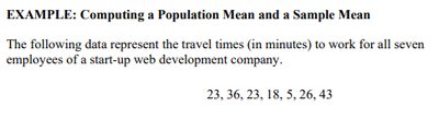
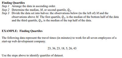
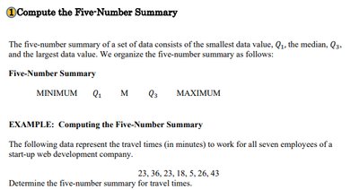
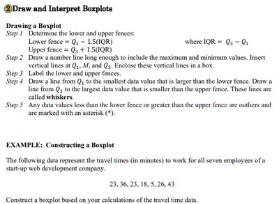
Example: Travel times (in minutes) for seven employees: 23, 36, 23, 18, 5, 26, 43.

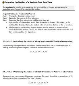
Median

The median is the value that lies in the middle of the data when arranged in ascending order. It is denoted by $M$.

• Arrange data in ascending order.

• If the number of observations is odd, the median is the middle value.

• If even, the median is the average of the two middle values.

Example: Median for 23, 36, 23, 18, 5, 26, 43 (odd number of observations).

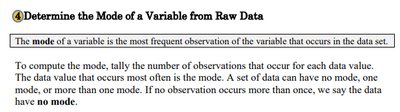
Mode

The mode is the most frequent observation in a data set. A data set may have no mode, one mode, or multiple modes.

• Tally the frequency of each data value.

• The value with the highest frequency is the mode.

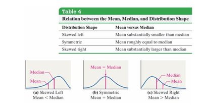
Relation Between Mean, Median, and Distribution Shape

The relationship between the mean and median can indicate the shape of a distribution:

Distribution Shape	Mean vs Median
Skewed left	Mean substantially smaller than median
Symmetric	Mean roughly equal to median
Skewed right	Mean substantially larger than median

Measures of Dispersion

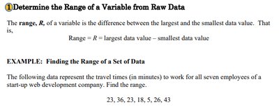
Range

The range ($R$) is the difference between the largest and smallest data values.

• Formula: $R = \text{largest data value} - \text{smallest data value}$

Example: Range for 23, 36, 23, 18, 5, 26, 43.

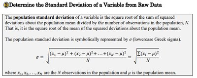
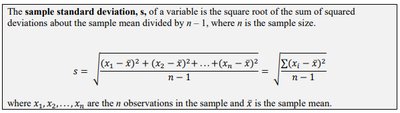
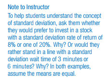
Standard Deviation

The standard deviation measures the spread of data values around the mean. It is the square root of the mean of squared deviations.

• Population Standard Deviation: $\sigma = \sqrt{\frac{\sum (x_i - \mu)^2}{N}}$

• Sample Standard Deviation: $s = \sqrt{\frac{\sum (x_i - \overline{x})^2}{n-1}}$

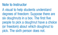
Degrees of Freedom

Degrees of freedom refer to the number of values that are free to vary in a calculation. For sample standard deviation, $n-1$ is used because one value is determined by the others.

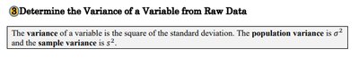
Variance

The variance is the square of the standard deviation. The population variance is $\sigma^2$ and the sample variance is $s^2$.

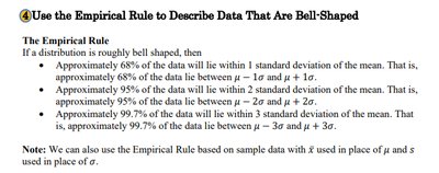
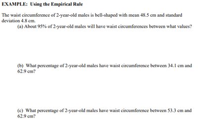
Empirical Rule for Bell-Shaped Data

The Empirical Rule describes the spread of data in a normal (bell-shaped) distribution:

• Approximately 68% of data within 1 standard deviation of the mean

• Approximately 95% within 2 standard deviations

• Approximately 99.7% within 3 standard deviations

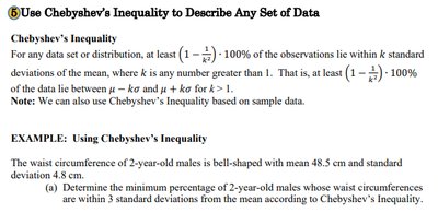
Chebyshev's Inequality

Chebyshev's Inequality applies to any data set, stating that at least $\left(1 - \frac{1}{k^2}\right) \times 100\%$ of observations lie within $k$ standard deviations of the mean, for $k > 1$.

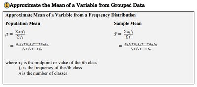
Grouped Data

Approximating the Mean from Grouped Data

When data is grouped, the mean can be approximated using class midpoints and frequencies:

• Population Mean: $\mu = \frac{\sum x_i f_i}{\sum f_i}$

• Sample Mean: $\overline{x} = \frac{\sum x_i f_i}{\sum f_i}$

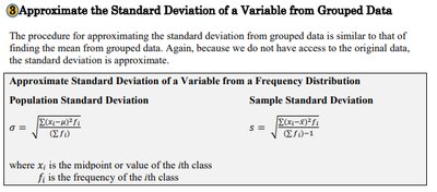
Approximating the Standard Deviation from Grouped Data

Standard deviation for grouped data is approximated using class midpoints and frequencies:

• Population Standard Deviation: $\sigma = \sqrt{\frac{\sum (x_i - \mu)^2 f_i}{\sum f_i}}$

• Sample Standard Deviation: $s = \sqrt{\frac{\sum (x_i - \overline{x})^2 f_i}{\sum f_i - 1}}$

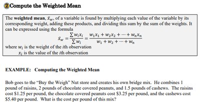
Weighted Mean

The weighted mean is calculated by multiplying each value by its weight, summing these products, and dividing by the sum of the weights:

• Formula: $\overline{x}_w = \frac{\sum w_i x_i}{\sum w_i}$

Measures of Position

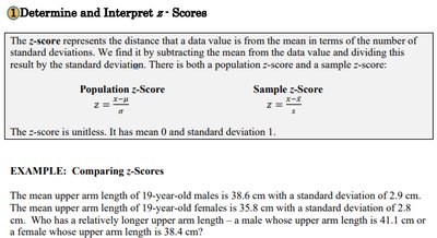
z-Scores

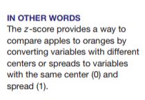
A z-score measures the distance of a data value from the mean in terms of standard deviations. It standardizes values for comparison.

• Population z-score: $z = \frac{x - \mu}{\sigma}$

• Sample z-score: $z = \frac{x - \overline{x}}{s}$

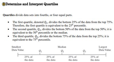
Quartiles

Quartiles divide data into four equal parts:

• $Q_1$: 25th percentile

• $Q_2$: 50th percentile (median)

• $Q_3$: 75th percentile

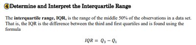
Interquartile Range (IQR)

The interquartile range (IQR) is the range of the middle 50% of observations:

• Formula: $\text{IQR} = Q_3 - Q_1$

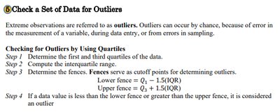
Outliers

Outliers are extreme observations. They are identified using quartiles and the IQR:

• Lower fence: $Q_1 - 1.5 \times \text{IQR}$

• Upper fence: $Q_3 + 1.5 \times \text{IQR}$

• Values outside these fences are considered outliers.

Five-Number Summary and Boxplots

Five-Number Summary

The five-number summary consists of the minimum, $Q_1$, median ($M$), $Q_3$, and maximum values.

Boxplots

Boxplots visually display the five-number summary and identify outliers. Steps to construct a boxplot:

• Determine lower and upper fences

• Draw a box from $Q_1$ to $Q_3$

• Draw lines (whiskers) to minimum and maximum values within fences

• Mark outliers with asterisks

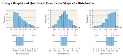
Summary Table: Distribution Shape and Measures

Boxplots and quartiles can be used to describe the shape of a distribution:

• Skewed right: Median < Mean

• Symmetric: Median = Mean

• Skewed left: Median > Mean