Chapter 3: Numerically Summarizing Data – Study Guide

Measures of Central Tendency

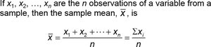
Arithmetic Mean

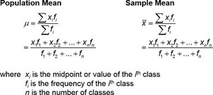
The arithmetic mean is a measure of central tendency that represents the average value of a variable in a data set. It is calculated by summing all values and dividing by the number of observations.

• Population Mean (μ): Uses all individuals in a population and is considered a parameter.

• Sample Mean (\(\bar{x}\)): Uses a subset (sample) of the population and is considered a statistic.

• Formula:

$\bar{x} = \frac{x_1 + x_2 + \cdots + x_n}{n} = \frac{\sum x_i}{n}$

• Example: Exam scores of 10 students can be used to compute both population and sample means.

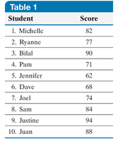
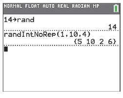
To find the sample mean, select a random sample and apply the formula above.

Median

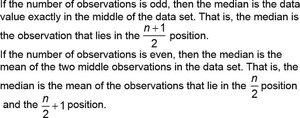
The median is the value that lies in the middle of the data when arranged in ascending order. It divides the data into two equal halves.

• Steps to Find Median:

• Arrange data in ascending order.

• Determine the number of observations, n.

• If n is odd, median is the value at position $\frac{n+1}{2}$.

• If n is even, median is the mean of values at positions $\frac{n}{2}$ and $\frac{n}{2}+1$.

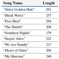
• Example: Median length of songs released in the 1970s.

Resistance of Statistics

A statistic is resistant if extreme values (outliers) do not affect its value substantially. The median is resistant, while the mean is not.

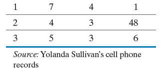
• Example: Comparing mean and median for cell phone call lengths.

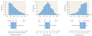
• For skewed distributions, the median is a better measure of central tendency.

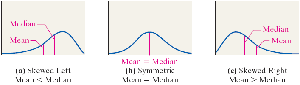
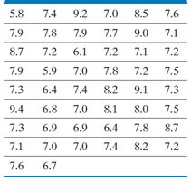
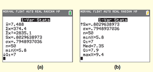
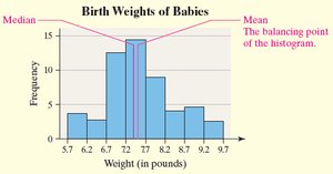
• Example: Birth weights of babies – mean and median are close, indicating a bell-shaped distribution.

Mode

The mode is the most frequent observation in a data set. Data can have no mode, one mode, or multiple modes.

• Example: Number of O-ring failures on space shuttle flights.

• Mode is 0, as it occurs most frequently.

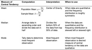
Comparison Table: Measures of Central Tendency

Measure	Computation	Interpretation	When to Use
Mean	Population: $\mu = \frac{\sum x_i}{N}$ Sample: $\bar{x} = \frac{\sum x_i}{n}$	Center of Gravity	Quantitative, symmetric distribution
Median	Arrange data, divide in half	Divides bottom 50% from top 50%	Quantitative, skewed distribution
Mode	Tally most frequent observation	Most frequent observation	Qualitative or when mode is desired

Measures of Dispersion

Range

The range is the difference between the largest and smallest data values.

• Formula: $R = \text{Largest Data Value} - \text{Smallest Data Value}$

• Example: Exam scores: $R = 94 - 62 = 32$ points

Standard Deviation

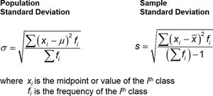
The standard deviation measures the spread of data values around the mean.

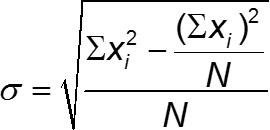
• Population Standard Deviation (σ):

$\sigma = \sqrt{\frac{\sum (x_i - \mu)^2}{N}}$

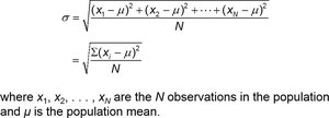
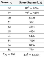
Computational formula:

$\sigma = \sqrt{\frac{\sum x_i^2 - (\sum x_i)^2 / N}{N}}$

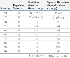
• Example: Calculating standard deviation for exam scores.

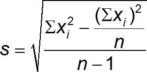
• Sample Standard Deviation (s):

$s = \sqrt{\frac{\sum (x_i - \bar{x})^2}{n-1}}$

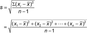
Computational formula:

$s = \sqrt{\frac{\sum x_i^2 - (\sum x_i)^2 / n}{n-1}}$

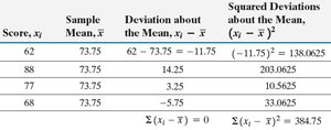
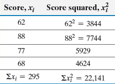
• Example: Calculating sample standard deviation for a random sample.

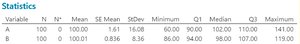
• Comparison: Standard deviation is larger for University A (16.1) than for University B (8.4), indicating more dispersion in University A.

Variance

The variance is the square of the standard deviation.

• Population Variance: $\sigma^2$

• Sample Variance: $s^2$

• Example: If $\sigma = 9.8$, then $\sigma^2 = 96.04$; if $s = 11.3$, then $s^2 = 127.7$

Empirical Rule (Bell-Shaped Distributions)

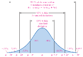
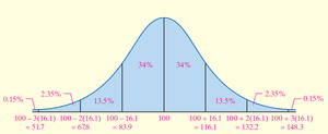
The Empirical Rule describes the spread of data in a bell-shaped (normal) distribution:

• 68% of data within 1 standard deviation of the mean

• 95% within 2 standard deviations

• 99.7% within 3 standard deviations

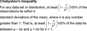
Chebyshev’s Inequality

Chebyshev’s Inequality applies to any data set, regardless of shape. It states that at least $1 - \frac{1}{k^2}$ of the data lies within k standard deviations of the mean, for $k > 1$.

$\text{At least } 1 - \frac{1}{k^2} \text{ of the data lies between } \mu - k\sigma \text{ and } \mu + k\sigma$

Grouped Data: Central Tendency and Dispersion

Mean from Grouped Data

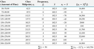
When only grouped data (frequency distributions) are available, the mean can be approximated using class midpoints and frequencies.

$\mu = \frac{\sum x_i f_i}{\sum f_i}$

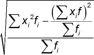
Standard Deviation from Grouped Data

Standard deviation can also be approximated from grouped data using midpoints and frequencies.

$\sigma = \sqrt{\frac{\sum (x_i - \mu)^2 f_i}{\sum f_i}}$

Computational formula:

$\sqrt{\frac{\sum x_i^2 f_i - (\sum x_i f_i)^2 / \sum f_i}{\sum f_i}}$

• Example: Parking and camera violation fines in NYC.

Measures of Position and Outliers

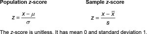
z-Scores

A z-score measures how many standard deviations a data value is from the mean.

• Population z-score: $z = \frac{x - \mu}{\sigma}$

• Sample z-score: $z = \frac{x - \bar{x}}{s}$

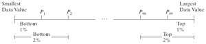
Percentiles

The kth percentile is the value below which k percent of the data falls.

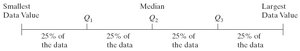
Quartiles

Quartiles divide data into four equal parts:

• Q1: 25th percentile

• Q2: 50th percentile (median)

• Q3: 75th percentile

Interquartile Range (IQR)

The interquartile range is the range of the middle 50% of the data:

$\text{IQR} = Q_3 - Q_1$

Outliers

To check for outliers:

• Compute lower fence: $Q_1 - 1.5 \times \text{IQR}$

• Compute upper fence: $Q_3 + 1.5 \times \text{IQR}$

• Values outside these fences are outliers.

Five-Number Summary and Boxplots

Five-Number Summary

The five-number summary consists of: minimum, Q1, median, Q3, maximum.

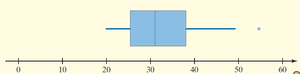
Boxplots

Boxplots visually display the five-number summary and identify outliers.

• Draw a box from Q1 to Q3, with a line at the median.

• Whiskers extend to the smallest and largest values within the fences.

• Outliers are marked with asterisks.

• Boxplots and quartiles can be used to describe the shape of a distribution.