Chapter 3: Numerically Summarizing Data – Study Guide

Measures of Central Tendency

Arithmetic Mean

The arithmetic mean is a measure of central tendency that represents the average value of a data set. It is calculated by summing all values and dividing by the number of observations. The mean is used for quantitative data and is most appropriate when the distribution is symmetric.

• Population Mean (μ): $\mu = \frac{\sum x_i}{N}$

• Sample Mean (x̄): $\bar{x} = \frac{\sum x_i}{n}$

• Interpretation: The mean is the "center of gravity" of the data.

• Example: For travel times: 23, 36, 23, 18, 5, 26, 43, the population mean is $\mu = \frac{23+36+23+18+5+26+43}{7} = 24.857$ minutes.

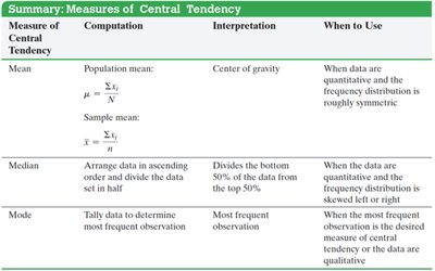
Median

The median is the middle value when data are arranged in ascending order. It divides the data into two equal halves and is resistant to extreme values.

• Computation: Arrange data, find the middle value (if odd n), or average the two middle values (if even n).

• Interpretation: Divides the bottom 50% from the top 50%.

• When to Use: When the data are skewed left or right.

Mode

The mode is the most frequent observation in a data set. It is useful for both quantitative and qualitative data.

• Computation: Tally the frequency of each value; the value with the highest frequency is the mode.

• Interpretation: Most frequent observation.

• When to Use: When the most frequent observation is desired or for qualitative data.

Resistance of Statistics

A statistic is resistant if it is not affected substantially by extreme values. The median is resistant, while the mean is not.

• Example: Adding an extreme value (e.g., 70 minutes) to the travel time data increases the mean significantly, but the median changes less.

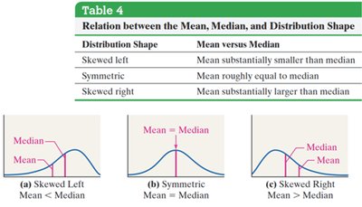
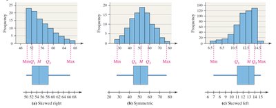
Relation Between Mean, Median, and Distribution Shape

The relationship between the mean and median provides insight into the shape of the distribution:

• Skewed left: Mean < Median

• Symmetric: Mean ≈ Median

• Skewed right: Mean > Median

Measures of Dispersion

Range

The range is the difference between the largest and smallest values in a data set.

• Formula: $R = \text{largest value} - \text{smallest value}$

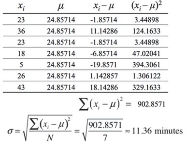
Standard Deviation

The standard deviation measures the average distance of data values from the mean. It quantifies the spread of the data.

• Population Standard Deviation (σ): $\sigma = \sqrt{\frac{\sum (x_i - \mu)^2}{N}}$

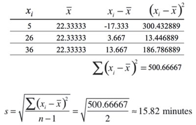
• Sample Standard Deviation (s): $s = \sqrt{\frac{\sum (x_i - \bar{x})^2}{n-1}}$

• Degrees of Freedom: n-1 for sample standard deviation.

• Example: For travel times, population standard deviation is $\sigma \approx 11.36$ minutes.

Variance

The variance is the square of the standard deviation and measures the average squared deviation from the mean.

• Population Variance: $\sigma^2$

• Sample Variance: $s^2$

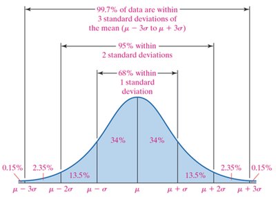
The Empirical Rule

The Empirical Rule describes the spread of data in a bell-shaped (normal) distribution:

• 68% of data within 1 standard deviation of the mean

• 95% within 2 standard deviations

• 99.7% within 3 standard deviations

Chebyshev’s Inequality

Chebyshev’s Inequality applies to any data set, regardless of shape. It states that at least $1 - \frac{1}{k^2}$ of the data lie within k standard deviations of the mean (for k > 1).

• Formula: $1 - \frac{1}{k^2}$

• Application: Minimum percentage of data within k standard deviations.

Measures from Grouped Data

Approximate Mean from Grouped Data

When only grouped data are available, the mean can be approximated using class midpoints and frequencies.

• Formula: $\mu \approx \frac{\sum x_i f_i}{\sum f_i}$

Weighted Mean

The weighted mean accounts for values with different weights.

• Formula: $\bar{x}_w = \frac{\sum w_i x_i}{\sum w_i}$

Approximate Standard Deviation from Grouped Data

Standard deviation can be approximated from grouped data using class midpoints and frequencies.

• Formula: $\sigma \approx \sqrt{\frac{\sum f_i (x_i - \mu)^2}{\sum f_i}}$

Measures of Position and Outliers

z-Scores

A z-score measures how many standard deviations a data value is from the mean.

• Population z-score: $z = \frac{x - \mu}{\sigma}$

• Sample z-score: $z = \frac{x - \bar{x}}{s}$

• Interpretation: z-scores are unitless and have mean 0, standard deviation 1.

Percentiles

The kth percentile is the value below which k percent of the data fall.

• Interpretation: Useful for comparing relative standing in a data set.

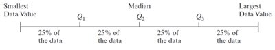
Quartiles

Quartiles divide the data into four equal parts:

• Q1: 25th percentile

• Q2: 50th percentile (median)

• Q3: 75th percentile

Interquartile Range (IQR)

The interquartile range (IQR) measures the spread of the middle 50% of the data.

• Formula: $\text{IQR} = Q_3 - Q_1$

Checking for Outliers

Outliers are extreme values that fall outside the expected range. They can be identified using quartiles and the IQR:

• Lower fence: $Q_1 - 1.5 \times \text{IQR}$

• Upper fence: $Q_3 + 1.5 \times \text{IQR}$

• Values outside these fences are considered outliers.

The Five-Number Summary and Boxplots

Five-Number Summary

The five-number summary consists of:

• Minimum

• Q1

• Median (Q2)

• Q3

• Maximum

Boxplots

Boxplots visually display the five-number summary and highlight outliers. They are useful for comparing distributions.

• Box extends from Q1 to Q3, with a line at the median.

• Whiskers extend to the smallest and largest values within the fences.

• Outliers are marked with asterisks.

Summary: Which Measures to Report

• Symmetric distribution: Report mean and standard deviation.

• Skewed distribution: Report median and interquartile range.