Chapter 5: Probability in Our Daily Lives – Structured Study Notes

Probability in Our Daily Lives

Introduction to Probability

Probability is the mathematical framework for quantifying uncertainty and making informed decisions in the presence of randomness. It allows us to predict the long-term behavior of random phenomena, even though individual outcomes may be unpredictable in the short run.

• Chance behavior is unpredictable in the short run but follows a regular and predictable pattern in the long run.

• A random phenomenon is one where individual outcomes are uncertain, but a regular distribution of outcomes emerges over many repetitions.

• The probability of an outcome is the proportion of times that outcome would occur in a very long series of repetitions.

Section 5.1: How Probability Quantifies Randomness

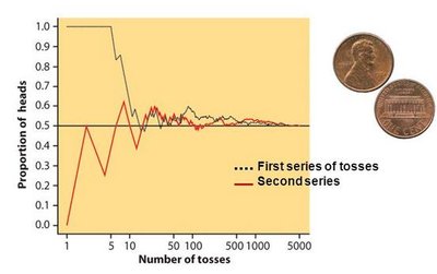
Long-Run Behavior and the Law of Large Numbers

Random phenomena exhibit high variability in the short run, but their long-term behavior is predictable. The law of large numbers, first formalized by Jacob Bernoulli, states that as the number of trials increases, the proportion of occurrences of any given outcome approaches a specific value (the probability).

• Each trial must be independent: the outcome of one trial does not affect another.

• The law of large numbers guarantees long-run regularity, not short-run predictability.

• Casinos and insurance companies rely on this law for long-term profit, despite short-term variability.

Empirical probability is the sample proportion used to estimate the actual probability based on observed data.

Types of Probability

• Relative frequency probability: Based on the long-run proportion of times an event occurs in repeated trials.

• Subjective probability: Based on personal judgment or belief, used when historical data is unavailable. Bayesian statistics is a branch that uses subjective probability.

• Subjective probabilities of 0 or 1 are generally considered unreliable unless the event is impossible or certain.

Section 5.2: Finding Probabilities

Basic Terminology

• Sample space (S): The set of all possible outcomes of a random phenomenon.

• Event: Any outcome or set of outcomes (subset of the sample space).

• Probability model: A mathematical description consisting of a sample space and a rule for assigning probabilities to events.

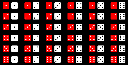
Example: Rolling one fair die: S = {1, 2, 3, 4, 5, 6}

Example: Tossing three fair coins: S = {HHH, HHT, HTH, HTT, THH, THT, TTH, TTT}

Rules for Probabilities in a Sample Space

• The probability of each individual outcome is between 0 and 1: $0 \leq P(A) \leq 1$

• The sum of the probabilities of all possible outcomes is 1: $P(S) = 1$

Probability of an Event (Equally Likely Outcomes)

When all outcomes are equally likely:

$P(A) = \frac{\text{number of outcomes in event A}}{\text{number of outcomes in the sample space}}$

Note: Equally likely outcomes are rare in real-world scenarios.

Visualizing Events: Venn Diagrams

Venn diagrams are useful for representing sample spaces and events, especially when analyzing unions, intersections, and complements.

Example: Probability with Two Dice

When rolling two fair dice, the sample space consists of all ordered pairs (i, j) where i and j are integers from 1 to 6. For example, the probability that the sum is 7 can be found by counting the number of pairs that sum to 7 and dividing by 36 (the total number of outcomes).

Section 5.3: Basic Rules for Finding Probabilities About a Pair of Events

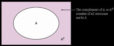
Complements

The complement of an event A (denoted Ac) consists of all outcomes in the sample space that are not in A. The probability that an event does not occur is:

$P(A^c) = 1 - P(A)$

This is useful when it is easier to calculate the probability of the complement rather than the event itself.

Disjoint (Mutually Exclusive) Events

Two events are disjoint if they have no outcomes in common and cannot occur simultaneously.

• Example: Rolling a die: A = {even numbers}, B = {odd numbers}. A and B are disjoint.

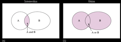
Unions and Intersections

• The intersection of events A and B (A ∩ B): outcomes in both A and B.

• The union of events A and B (A ∪ B): outcomes in A or B or both.

Cues: 'Or' indicates union; 'and' indicates intersection.

Addition Rule for Probabilities

For any two events A and B:

$P(A \text{ or } B) = P(A) + P(B) - P(A \text{ and } B)$

or

$P(A \cup B) = P(A) + P(B) - P(A \cap B)$

If A and B are disjoint:

$P(A \text{ or } B) = P(A) + P(B)$

Example: Newspaper Reading

Suppose 65% of students read Paper 1, 51% read Paper 2, and 27% read both. The probability a student reads at least one is:

$P(\text{at least one}) = 0.65 + 0.51 - 0.27 = 0.89$

Example: Student Classification Probability Model

Classification	First-Year	Sophomore	Junior	Senior	Graduate
Probability	0.25	0.22	0.23	0.20	0.10

• Probability not a graduate student: $1 - 0.10 = 0.90$

• Probability first-year or sophomore: $0.25 + 0.22 = 0.47$

Section 5.4: Multiplication Rule for Independent Events

Multiplication Rule

For two independent events A and B (the occurrence of one does not affect the other):

$P(A \text{ and } B) = P(A) \times P(B)$

or

$P(A \cap B) = P(A) \times P(B)$

• Example: Probability of rolling a 6 on each of two dice: $P(6 \text{ on die 1}) = 1/6$, $P(6 \text{ on die 2}) = 1/6$, so $P(6 \text{ on both}) = 1/6 \times 1/6 = 1/36$

Note: Do not assume independence unless justified by the context.

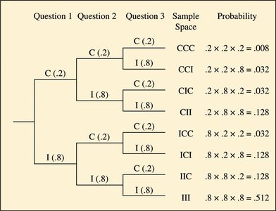
Tree Diagrams

Tree diagrams help visualize all possible outcomes and their probabilities, especially for sequential events.

Odds

Odds are defined as the probability that an event will occur divided by the probability that it will not occur:

$\text{Odds in favor} = \frac{P(\text{event})}{1 - P(\text{event})}$

• Example: If $P(\text{win}) = 0.4$, odds in favor = $0.4 / 0.6 = 2/3$

Summary: Rules for Finding Probabilities

• The probability of each individual outcome is between 0 and 1, and the total probability is 1.

• The probability of an event is the sum of the probabilities of the outcomes in that event.

• For an event A and its complement Ac: $P(A^c) = 1 - P(A)$

• For the union of two events: $P(A \cup B) = P(A) + P(B) - P(A \cap B)$

• If A and B are disjoint: $P(A \cup B) = P(A) + P(B)$

• For independent events: $P(A \cap B) = P(A) \times P(B)$

Additional info: Sections 5.3 and 5.4 are not covered in detail in the original notes, but the above summary provides the essential rules and context for probability calculations.