Chapter 6 Study Guide

Normal Probability Distributions

The Standard Normal Distribution

The standard normal distribution is a continuous, bell-shaped, and symmetric probability distribution centered at a mean of 0 and a standard deviation of 1. It is used as a reference for all normal distributions, allowing probabilities to be calculated using standardized values called z-scores.

• Probability as Area: For continuous distributions, probability is represented by the area under the density curve. The total area under the curve is 1.

• Density Curve: The graph of a continuous probability distribution is called a density curve.

• z-score: $z = \frac{x - \mu}{\sigma}$, where x is the observed value, μ is the mean, and σ is the standard deviation.

• Interpretation: z < 0 means below the mean, z = 0 at the mean, z > 0 above the mean.

Example: If exam scores are normally distributed with μ = 74 and σ = 8, the z-score for a score of 85 is $z = \frac{85 - 74}{8} = 1.375$.

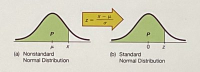
Using Table A-2: Finding Probabilities

Table A-2 provides cumulative probabilities (areas) from the left for given z-scores. To find probabilities:

• Area to the Left: P(Z < z) is found directly from the table.

• Area to the Right: Use the complement rule: P(Z > z) = 1 - P(Z < z).

• Area Between Two z-scores: Subtract the smaller cumulative area from the larger: P(a < Z < b) = P(Z < b) - P(Z < a).

• Working Backward: Given a probability, find the corresponding z-score by locating the area in the table and matching it to the z value.

Example: To find P(Z < 1.27), locate row 1.2 and column .07 in Table A-2. The intersection gives 0.8980, meaning about 89.8% of values fall below z = 1.27.

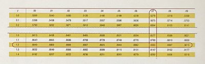
Critical Values and Percentiles

Critical values (zα) are z-scores with a specified area α to their right. For example, z0.025 is the z-score with 0.025 area to the right, commonly used in confidence intervals.

• Percentile: The value below which a given percentage of observations fall. To find the raw value for a percentile, use the z-score and convert back: $x = \mu + z\sigma$.

Example: The 90th percentile for exam scores with μ = 74 and σ = 8 is $x = 74 + (1.28)(8) = 84.24$.

Real Applications of Normal Distributions

Standardizing Raw Values

To use the standard normal distribution for real-world variables, convert raw values to z-scores. This process is called standardization and allows comparison across different normal distributions.

• Raw Value (x): The original measurement in its units.

• Standardized Value (z): The number of standard deviations x is from the mean.

• Formula: $z = \frac{x - \mu}{\sigma}$

• Reverse Conversion: $x = \mu + z\sigma$

Example: If plant heights are normally distributed with μ = 29 cm and σ = 2 cm, a height of 33 cm has $z = \frac{33 - 29}{2} = 2$.

Probability and Percentile Calculations

• To find the probability above a raw score, standardize the value, use Table A-2, and interpret the result in context.

• To find the raw value for a given percentile, find the z-score for the cumulative area, then convert back to x.

Example: For exam scores μ = 74, σ = 8, P(X > 85): $z = \frac{85 - 74}{8} = 1.38$, Table A-2 gives P(Z < 1.38) = 0.9162, so P(X > 85) = 1 - 0.9162 = 0.0838.

Sampling Distributions and Estimators

Sampling Distributions

A sampling distribution is the probability distribution of a statistic (such as the mean, proportion, or variance) calculated from all possible samples of a given size from the same population.

• Sampling Variability: Sample statistics vary from sample to sample due to random selection.

• Three Distributions:

  • Population Distribution: Distribution of all individual values in the population.

  • Sample Distribution: Distribution of values in one random sample.

  • Sampling Distribution: Distribution of a statistic across all possible samples.

Example: If plant heights are measured for many samples of n = 25, the distribution of sample means x̄ forms the sampling distribution of x̄.

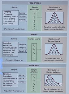
Estimators and Unbiasedness

An estimator is a statistic used to estimate a population parameter. An estimator is unbiased if its sampling distribution is centered at the parameter it estimates.

• Sample Mean (x̄): Unbiased estimator of population mean μ.

• Sample Proportion (p̂): Unbiased estimator of population proportion p.

• Sample Variance (s²): Unbiased estimator of population variance σ².

• Sample Standard Deviation (s): Slightly biased downward estimator of σ.

Example: If the true population variance is σ² = 25, the average sample variance s² across many samples will equal 25, but the average sample standard deviation s will be slightly less than 5.

The Central Limit Theorem (CLT)

Properties of the Sampling Distribution of the Sample Mean

The Central Limit Theorem states that the sampling distribution of the sample mean x̄ becomes approximately normal as the sample size n increases, regardless of the population's shape.

• Center: The mean of the sampling distribution of x̄ is μ.

• Spread: The standard error of the mean is $\sigma_{\bar{x}} = \frac{\sigma}{\sqrt{n}}$.

• Shape: If the population is normal, the sampling distribution is normal for any n. If not, n ≥ 30 is sufficient for approximate normality.

Example: For σ = 12 and n = 36, $\sigma_{\bar{x}} = \frac{12}{6} = 2$.

Distinguishing Between Individual Observations and Sample Means

• Individual Observation (X): Use $z = \frac{x - \mu}{\sigma}$.

• Sample Mean (x̄): Use $z = \frac{\bar{x} - \mu}{\sigma / \sqrt{n}}$.

Example: For fish lengths μ = 30 cm, σ = 4 cm, n = 16, the probability that x̄ > 34 cm is much smaller than the probability that X > 34 cm due to reduced spread.

Assessing Normality

Using Histograms and Q-Q Plots

To determine if a normal model is reasonable for a population, use graphical displays:

• Histogram: Should be roughly symmetric, unimodal, and bell-shaped.

• Normal Q-Q Plot: Points should fall close to a straight line without systematic curvature.

• Outliers: Investigate unusual observations before discarding them.

Example: If a histogram of leaf lengths is bell-shaped and the Q-Q plot is linear, normality is reasonable.

Summary Table: Sampling Distributions

Statistic	Estimator	Unbiased?	Distribution Shape
Mean	x̄ estimates μ	Yes	Normal (or approx. normal for n ≥ 30)
Proportion	p̂ estimates p	Yes	Normal (as n increases)
Variance	s² estimates σ²	Yes	Right-skewed
Standard deviation	s estimates σ	No (slightly downward)	Right-skewed

Additional info: The images included reinforce the concepts of standardization, use of z-tables, and the behavior of sampling distributions for proportions, means, and variances.