Chapter 6: The Normal Probability Distribution – Study Notes

6.1 Properties of the Normal Distribution

Discrete vs. Continuous Random Variables

In statistics, random variables can be classified as either discrete or continuous. Discrete random variables have a finite or countable number of possible outcomes, while continuous random variables can take on an infinite number of values within a given interval.

• Discrete random variable: Example – Number of heads in 10 coin tosses.

• Continuous random variable: Example – The exact time a friend arrives, measured in minutes and seconds.

Uniform Distribution

A uniform distribution is a type of probability distribution in which all intervals of the same length within the range are equally likely. For example, if a friend can arrive anytime between 0 and 30 minutes late, and each minute is equally likely, the waiting time follows a uniform distribution.

• Probability Density Function (pdf): For a continuous random variable, the probability that the variable falls within a certain interval is given by the area under the curve of its pdf over that interval.

• Probability for exact values: For continuous variables, the probability of observing any exact value (e.g., exactly 12.89 minutes late) is zero.

Example: If X is uniformly distributed between 0 and 30, the probability that X is between 10 and 20 is proportional to the length of the interval (10 minutes out of 30, so probability = 10/30 = 1/3).

The Normal Distribution

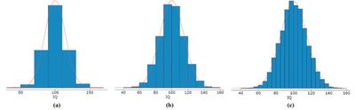
The normal distribution is a continuous probability distribution that is symmetric and bell-shaped. Many natural phenomena, such as IQ scores and birth weights, are approximately normally distributed. As sample size increases, the histogram of observed values approaches a smooth curve known as the normal curve.

• Definition: A continuous random variable is normally distributed if its probability distribution follows the bell-shaped normal curve.

Properties of the Normal Curve

To define a normal distribution, we need the mean (μ) and standard deviation (σ):

• The curve is symmetric about the mean μ.

• The highest point occurs at the mean.

• The spread is determined by the standard deviation σ.

• The total area under the curve is 1.

• As you move further from the mean, the curve approaches (but never touches) the horizontal axis.

• Empirical Rule: Approximately 68% of data falls within 1σ, 95% within 2σ, and 99.7% within 3σ of the mean.

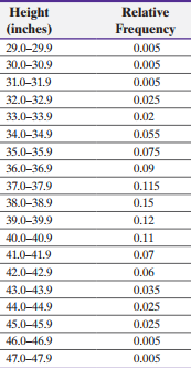
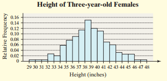
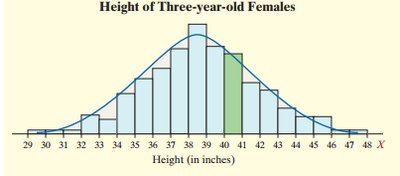
Example: The table below shows the relative frequency distribution of heights for three-year-old females. The mean is μ = 38.72 inches, σ = 3.17 inches.

Height (inches)	Relative Frequency
29.0–29.9	0.005
30.0–30.9	0.005
31.0–31.9	0.005
32.0–32.9	0.02
33.0–33.9	0.025
34.0–34.9	0.055
35.0–35.9	0.075
36.0–36.9	0.09
37.0–37.9	0.115
38.0–38.9	0.15
39.0–39.9	0.12
40.0–40.9	0.11
41.0–41.9	0.07
42.0–42.9	0.035
43.0–43.9	0.025
44.0–44.9	0.02
45.0–45.9	0.005
46.0–46.9	0.005
47.0–47.9	0.005

The normal curve can be described by the following probability density function (pdf):

$f(x) = \frac{1}{\sigma \sqrt{2\pi}} e^{-\frac{1}{2} \left( \frac{x-\mu}{\sigma} \right)^2}$

Additional info: This formula is not typically used directly in introductory statistics, but it underlies all normal probability calculations.

Area Under a Normal Curve

The area under the normal curve between two values represents the probability that the random variable falls within that interval. For a continuous variable, the probability of any exact value is zero: $P(X = a) = 0$.

• Example: If cholesterol levels are normally distributed with μ = 180 mg/dL and σ = 36.2 mg/dL, the area to the right of x = 200 represents the proportion of individuals with high cholesterol.

6.2 Applications of the Normal Distribution

Standardizing a Normal Random Variable

Any normal random variable X can be transformed into a standard normal variable Z (mean 0, standard deviation 1) using the formula:

$z = \frac{x - \mu}{\sigma}$

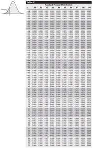
• This allows us to use standard normal tables (z-tables) to find probabilities.

• Example: For IQ scores with μ = 100, σ = 15, an individual with IQ = 120 has $z = (120-100)/15 = 1.33$.

Finding Areas Under the Normal Curve

To find probabilities for normal distributions:

1. Draw a normal curve and shade the desired area.

2. Convert the value(s) of x to z-score(s).

3. Use the z-table to find the area to the left of the z-score(s).

Common Problems:

• Area to the left of x: Use z-table directly.

• Area to the right of x: 1 minus area to the left.

• Area between x1 and x2: Area to left of z2 minus area to left of z1.

Example: SAT math scores are normally distributed with μ = 516, σ = 116. Find the probability a student scores less than 500, more than 600, or between 525 and 550.

Finding the Value of a Normal Random Variable

Given a probability (area), you can find the corresponding value of x:

1. Draw a normal curve and shade the desired area.

2. Use the z-table to find the z-score for the area.

3. Convert z to x using $x = \mu + z\sigma$.

Example: For heights of three-year-old females (μ = 38.72, σ = 3.17), find the height at the 20th percentile or the heights separating the middle 80% from the bottom and top 10%.

6.3 Assessing Normality

Using a Frequency Histogram

A frequency histogram is a graphical tool to assess if data is approximately normal. Look for:

• Bell-shaped curve with a single peak

• Rough symmetry (no strong skewness)

• Few outliers

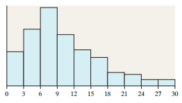
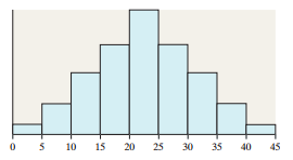
Example: Comparing wait times at two restaurants:

• Restaurant A: Skewed right, not normal

• Restaurant B: Bell-shaped, approximately normal

Using a Normal Probability Plot

A normal probability plot compares observed values to expected z-scores. If the data is normal, the points will form a straight line. This method is common in advanced statistics courses.