Chapter 7: Confidence Intervals and Estimation in Statistics

Chapter 7: Confidence Intervals and Estimation

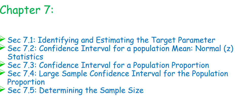
Sec 7.1: Identifying and Estimating the Target Parameter

In statistical inference, the target parameter is the population characteristic (such as the mean or proportion) that we aim to estimate using sample data. Identifying the correct parameter is crucial for selecting the appropriate estimation method.

• Parameter: A numerical summary of a population (e.g., population mean \( \mu \), population proportion \( p \)).

• Statistic: A numerical summary calculated from a sample (e.g., sample mean \( \overline{x} \), sample proportion \( \hat{p} \)).

• Point Estimate: A single value estimate of a population parameter (e.g., using \( \overline{x} \) to estimate \( \mu \)).

• Interval Estimate: A range of values (confidence interval) likely to contain the population parameter.

Example: If we want to estimate the average height of all college students, the target parameter is the population mean height \( \mu \).

Sec 7.2: Confidence Interval for a Population Mean: Normal (z) Statistics

A confidence interval provides a range of plausible values for a population mean, based on sample data. When the population standard deviation \( \sigma \) is known and the sample size is large (or the population is normal), the z-interval is used.

• Formula:

$\left( \overline{x} - z^* \frac{\sigma}{\sqrt{n}},\ \overline{x} + z^* \frac{\sigma}{\sqrt{n}} \right)$

• \( \overline{x} \): Sample mean

• \( z^* \): Critical value from the standard normal distribution for the desired confidence level

• \( \sigma \): Population standard deviation

• \( n \): Sample size

Example: For a 95% confidence interval, \( z^* \approx 1.96 \).

Sec 7.3: Confidence Interval for a Population Proportion

To estimate a population proportion \( p \), we use the sample proportion \( \hat{p} \) and construct a confidence interval.

• Formula:

$\left( \hat{p} - z^* \sqrt{\frac{\hat{p}(1-\hat{p})}{n}},\ \hat{p} + z^* \sqrt{\frac{\hat{p}(1-\hat{p})}{n}} \right)$

• \( \hat{p} \): Sample proportion

• \( n \): Sample size

• \( z^* \): Critical value for the desired confidence level

Example: If 60 out of 100 surveyed students prefer online classes, \( \hat{p} = 0.6 \).

Sec 7.4: Large Sample Confidence Interval for the Population Proportion

For large samples, the sampling distribution of \( \hat{p} \) is approximately normal (by the Central Limit Theorem), allowing the use of the normal (z) confidence interval for proportions. The rule of thumb is that both \( n\hat{p} \) and \( n(1-\hat{p}) \) should be at least 10.

• Formula (same as above):

$\left( \hat{p} - z^* \sqrt{\frac{\hat{p}(1-\hat{p})}{n}},\ \hat{p} + z^* \sqrt{\frac{\hat{p}(1-\hat{p})}{n}} \right)$

• Check: \( n\hat{p} \geq 10 \) and \( n(1-\hat{p}) \geq 10 \)

Example: In a poll of 200 people, 150 support a policy. \( \hat{p} = 0.75 \), \( n\hat{p} = 150 \), \( n(1-\hat{p}) = 50 \).

Sec 7.5: Determining the Sample Size

To achieve a desired margin of error in a confidence interval, we can calculate the required sample size before collecting data.

• For a mean:

$n = \left( \frac{z^* \sigma}{E} \right)^2$

• \( E \): Desired margin of error

• For a proportion:

$n = \frac{(z^*)^2 \hat{p}(1-\hat{p})}{E^2}$

• If no prior estimate for \( \hat{p} \), use \( \hat{p} = 0.5 \) for maximum sample size.

Example: To estimate a proportion with a margin of error of 0.03 at 95% confidence, \( z^* = 1.96 \), \( \hat{p} = 0.5 \):

$n = \frac{(1.96)^2 \times 0.5 \times 0.5}{0.03^2} \approx 1068$