Chapter 7: The Normal Probability Distribution – Study Notes

Chapter 7: The Normal Probability Distribution

7.1 Properties of the Normal Distribution

The normal probability distribution is a fundamental concept in statistics, describing many naturally occurring phenomena. This section introduces the uniform and normal distributions, their properties, and the significance of area under the curve.

Uniform Probability Distribution

• Definition: A uniform probability distribution is a continuous probability distribution where all intervals of the same length within the distribution's range are equally likely.

• Probability Density Function (pdf): An equation used to compute probabilities for continuous random variables. It must satisfy:

  • The total area under the graph over all possible values equals 1.

  • The height of the graph is always non-negative.

• Example: If a package is delivered between 10 am and 11 am, the probability of arrival in any 1-minute interval is the same for all intervals within that hour.

• Area Interpretation: The area under the pdf over an interval represents the probability that the random variable falls within that interval.

Normal Probability Distribution

• Definition: A normal distribution is a continuous probability distribution that is symmetric and bell-shaped, described by its mean (μ) and standard deviation (σ).

• Graphical Representation: As the class width in a histogram decreases, the histogram approaches the smooth, bell-shaped normal curve.

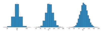
• Normal Curve: The normal curve is a model for distributions such as IQ scores or birth weights, where data is symmetrically distributed around the mean.

Properties of the Normal Curve

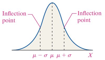
• The curve is symmetric about the mean, μ.

• Mean = median = mode; the highest point is at x = μ.

• Inflection points occur at μ - σ and μ + σ.

• Total area under the curve is 1.

• Area to the left and right of the mean is each 0.5.

• The curve approaches, but never touches, the horizontal axis as x → ±∞.

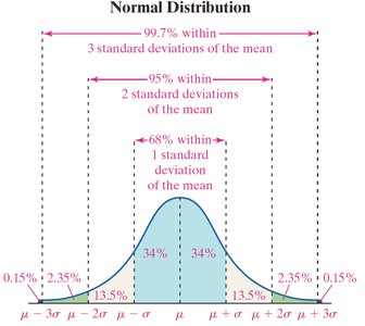
• The Empirical Rule:

  • ~68% of data within 1 standard deviation (μ ± σ)

  • ~95% within 2 standard deviations (μ ± 2σ)

  • ~99.7% within 3 standard deviations (μ ± 3σ)

  

The Role of Area in the Normal Density Function

• The area under the normal curve for an interval represents:

  • The proportion of the population with values in that interval

  • The probability that a randomly selected individual falls in that interval

• Example: If the area to the right of x = 450 feet under a normal curve for home run distances is 0.026, then 2.6% of home runs exceed 450 feet.

7.2 Applications of the Normal Distribution

This section covers how to find and interpret areas under the normal curve, and how to find values corresponding to given probabilities or percentiles.

Finding and Interpreting Area Under a Normal Curve

• Areas can be found using Z-tables or statistical software.

• Z-score: The number of standard deviations a value x is from the mean μ: $z = \frac{x - \mu}{\sigma}$

• Percentiles: The kth percentile is the value below which k% of the data falls.

• Example: If ball bearing diameters are normally distributed with μ = 1 cm, σ = 0.002 cm, the area under the curve between 0.995 and 1.005 cm gives the proportion meeting specifications.

Finding the Value of a Normal Random Variable

• Given a probability or percentile, use the Z-score and solve for x: $x = \mu + z\sigma$

• Example: To find the 90th percentile of home run distances (μ = 400.3 ft, σ = 25.6 ft), find the Z-score for the 90th percentile and solve for x.

7.3 Assessing Normality

Determining whether data is approximately normal is important for many statistical methods. This section introduces normal probability plots as a tool for this assessment.

Normal Probability Plots

• Purpose: To visually assess if a data set is approximately normally distributed.

• Construction Steps:

  1. Arrange data in ascending order.

  2. Compute expected proportions for each data point: $f_i = \frac{i - 0.375}{n + 0.25}$

  3. Find the Z-score corresponding to each $f_i$.

  4. Plot observed values (x-axis) vs. expected Z-scores (y-axis).

• If the plot is approximately linear, the data is likely normal.

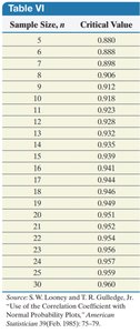
• Critical Value Table: The linear correlation coefficient between observed values and expected Z-scores should exceed a critical value for normality to be assumed.

7.4 The Normal Approximation to the Binomial Probability Distribution

When certain conditions are met, the binomial distribution can be approximated by the normal distribution, simplifying probability calculations for large samples.

Criteria for Binomial Experiments

• The experiment consists of n independent trials.

• Each trial has two outcomes: success or failure.

• The probability of success, p, is constant for each trial.

Normal Approximation Conditions

• If $np(1-p) \geq 10$, the binomial distribution is approximately normal.

• Mean: $\mu = np$

• Standard deviation: $\sigma = \sqrt{np(1-p)}$

Example Applications

• Calculating the probability of a certain number of successes in a large sample (e.g., flight cancellations, households buying gifts for pets) using the normal approximation.

Additional info:

• The normal approximation is especially useful when direct calculation of binomial probabilities is computationally intensive.