Chapter 7: The Normal Probability Distribution – Structured Study Notes

Normal Probability Distributions

Uniform Probability Distribution

The uniform probability distribution is a type of continuous probability distribution where all intervals of equal length within the distribution's range are equally likely. This is often used to model situations where every outcome in a given interval has the same probability.

• Probability Density Function (pdf): An equation used to compute probabilities for continuous random variables. It must satisfy:

  • The total area under the graph over all possible values equals 1.

  • The height of the graph is always greater than or equal to 0 for all possible values.

• Example: If a package is delivered between 10 am and 11 am, the probability of arrival in any 1-minute interval is equal. The random variable X (minutes after 10 am) follows a uniform distribution between 0 and 60.

• Area under the curve: The area under the pdf over an interval represents the probability of observing a value in that interval.

Normal Probability Distribution

The normal probability distribution is a continuous distribution characterized by its bell-shaped curve. Many natural phenomena, such as IQ scores and birth weights, follow this distribution.

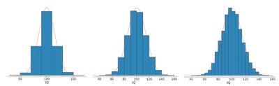
• Definition: A random variable is normally distributed if its relative frequency histogram has the shape of a normal curve.

• Graphical Representation: As the class width in a histogram decreases, the normal curve closely approximates the histogram.

Properties of the Normal Curve

The normal curve has several important properties that make it a fundamental concept in statistics.

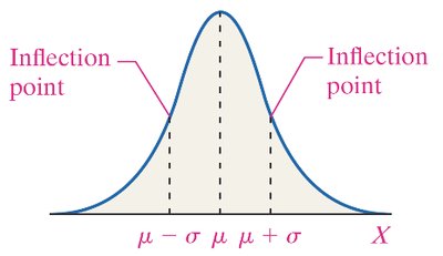
• Symmetry: The curve is symmetric about its mean, $\mu$.

• Single Peak: Mean = median = mode; the highest point occurs at $x = \mu$.

• Inflection Points: Occur at $\mu - \sigma$ and $\mu + \sigma$.

• Total Area: The area under the curve is 1.

• Equal Areas: The area to the left and right of the mean are both 0.5.

• Asymptotic: The curve approaches, but never touches, the horizontal axis as $x$ increases or decreases without bound.

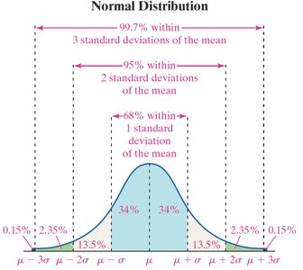
• Empirical Rule:

  • Approximately 68% of the area is between $\mu - \sigma$ and $\mu + \sigma$.

  • Approximately 95% is between $\mu - 2\sigma$ and $\mu + 2\sigma$.

  • Approximately 99.7% is between $\mu - 3\sigma$ and $\mu + 3\sigma$.

Role of Area in the Normal Density Function

The area under the normal curve for any interval represents the proportion of the population with a characteristic or the probability that a randomly selected individual will have that characteristic.

• Example: If the area to the right of $x = 450$ feet under a normal curve is 0.026, then:

  • 2.6% of home runs traveled more than 450 feet.

  • The probability that a randomly selected home run exceeded 450 feet is 0.026.

Applications of the Normal Distribution

Finding and Interpreting Area Under a Normal Curve

To find the area under a normal curve, use Z-scores and tables or technology. The area represents the probability or proportion of values within a specified interval.

• Z-score: $z = \frac{x - \mu}{\sigma}$

• Percentile Rank: The area under the curve to the left of a value gives its percentile rank.

• Example: If ball bearing diameters are normally distributed with mean 1 cm and standard deviation 0.002 cm, the area under the curve between 0.995 and 1.005 cm gives the proportion meeting specifications.

Finding the Value of a Normal Random Variable

Given a probability, proportion, or percentile rank, you can find the corresponding value of a normal random variable using the inverse of the Z-score formula.

• Inverse Z-score: $x = \mu + z\sigma$

• Example: To find the 90th percentile for home run distances with $\mu = 400.3$ feet and $\sigma = 25.6$ feet, use the Z-score for the 90th percentile and solve for $x$.

Assessing Normality

Normal Probability Plots

Normal probability plots are used to assess whether sample data comes from a normally distributed population, especially for small samples.

• Steps to Draw a Normal Probability Plot:

  1. Arrange data in ascending order.

  2. Compute expected proportion for each value: $f_i = \frac{i - 0.375}{n + 0.25}$

  3. Find the Z-score corresponding to $f_i$.

  4. Plot observed values (horizontal axis) vs. expected Z-scores (vertical axis).

• Interpretation: If the plot is approximately linear, the data is likely normally distributed.

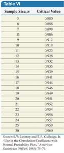
• Critical Value Table: Compare the linear correlation coefficient to the critical value for the sample size to assess normality.

Normal Approximation to the Binomial Probability Distribution

Criteria for Binomial Probability Experiment

A binomial experiment must satisfy:

• The experiment is performed n independent times (trials).

• Each trial has two mutually exclusive outcomes: success or failure.

• The probability of success, p, is the same for each trial.

Normal Approximation Criteria

If $np(1-p) \geq 10$, the binomial random variable X is approximately normally distributed.

• Mean: $\mu = np$

• Standard deviation: $\sigma = \sqrt{np(1-p)}$

Applications

• Example: If 8.5% of households buy their pet dog a gift for Valentine’s Day, in a sample of 200 households:

  • Expected number: $\mu = 200 \times 0.085 = 17$

  • Standard deviation: $\sigma = \sqrt{200 \times 0.085 \times 0.915}$

  • Probability calculations for more than 25 gifts use the normal approximation.

Tables and Data Interpretation

Critical Value Table for Normal Probability Plots

This table is used to determine if the linear correlation coefficient from a normal probability plot is sufficient to conclude normality for a given sample size.

Sample Size, n	Critical Value
5	0.880
6	0.888
7	0.898
8	0.906
9	0.912
10	0.918
11	0.922
12	0.928
13	0.932
14	0.939
15	0.941
16	0.944
17	0.946
18	0.948
19	0.950
20	0.951
21	0.952
22	0.954
23	0.955
24	0.957
25	0.958
30	0.960

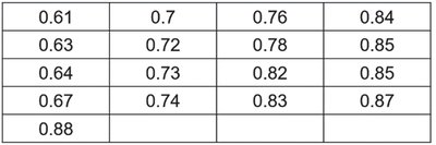
Additional Data Table

This table appears to show values for comparison or classification, possibly related to statistical measures or critical values. The exact context is not specified, but it may be used for reference in statistical calculations.

0.61	0.7	0.76	0.84
0.63	0.72	0.78	0.85
0.64	0.73	0.82	0.85
0.67	0.74	0.83	0.87
0.88

Additional info: The table may represent critical values or thresholds for statistical tests, but the exact application is not specified in the provided material.