Chapter 7: The Normal Probability Distribution – Study Notes

WeChapter 7: The Normal Probability Distribution

7.1 Properties of the Normal Distribution

The normal probability distribution is a fundamental concept in statistics, describing many naturally occurring phenomena. This section introduces the properties of the normal distribution, including its graphical representation and the role of area under the curve.

Uniform Probability Distribution

• Definition: A uniform probability distribution is a continuous probability distribution where all intervals of the same length within the distribution's range are equally probable.

• Probability Density Function (pdf): For a continuous random variable X, the pdf must satisfy:

  • The total area under the curve over all possible values equals 1.

  • The height of the curve is always non-negative.

• Example: If a package is delivered between 10:00 and 11:00 am, and X is the number of minutes after 10:00, then X is uniformly distributed on [0, 60].

• Area Interpretation: The probability that X falls within a certain interval is the area under the pdf over that interval.

Graphing a Normal Curve

Unlike the uniform distribution, many real-world variables (e.g., IQ scores, birth weights) are modeled by the normal distribution, which is bell-shaped and symmetric.

• Normal Distribution: A continuous random variable is normally distributed if its histogram is bell-shaped and symmetric.

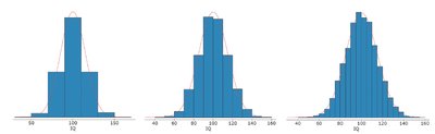
• Graphical Representation: As the class width in a histogram decreases, the histogram approaches the smooth normal curve.

Properties of the Normal Curve

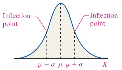
• Symmetry: The curve is symmetric about the mean (μ).

• Single Peak: Mean = median = mode; the highest point is at x = μ.

• Inflection Points: Located at μ - σ and μ + σ, where σ is the standard deviation.

• Total Area: The area under the curve is 1.

• Equal Halves: The area to the left and right of μ is each 0.5.

• Asymptotic: The curve approaches, but never touches, the horizontal axis as x → ±∞.

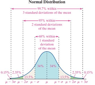
• Empirical Rule (68-95-99.7 Rule):

  • ~68% of data within 1σ of μ

  • ~95% within 2σ

  • ~99.7% within 3σ

The Role of Area in the Normal Density Function

• The area under the normal curve for an interval represents:

  • The proportion of the population with values in that interval

  • The probability that a randomly selected individual falls in that interval

• Example: If the area to the right of x = 450 feet under a normal curve is 0.026, then 2.6% of home runs exceed 450 feet.

7.2 Applications of the Normal Distribution

This section covers how to find and interpret areas under the normal curve, and how to find values corresponding to given probabilities or percentiles.

Finding and Interpreting Area Under a Normal Curve

• Areas under the curve can be found using Z-tables or technology.

• Percentile ranks can be determined from the area under the curve to the left of a value.

• Example: For ball bearings with diameters normally distributed (μ = 1 cm, σ = 0.002 cm), the probability a bearing is under 0.999 cm is the area to the left of 0.999.

Finding the Value of a Normal Random Variable

• Given a probability or percentile, use the normal distribution to find the corresponding value (inverse problem).

• Example: To find the 90th percentile of home run distances (μ = 400.3 ft, σ = 25.6 ft), find the value x such that the area to the left is 0.90.

7.3 Assessing Normality

Many statistical methods require the assumption of normality. This section discusses how to assess whether data are approximately normal, especially for small samples.

Normal Probability Plots

• A normal probability plot graphs observed data versus expected Z-scores (normal scores).

• If the plot is approximately linear, the data are likely from a normal distribution.

• Steps to Construct:

  1. Order data from smallest to largest.

  2. Compute expected cumulative proportions: $f_i = \frac{i - 0.375}{n + 0.25}$

  3. Find the Z-score for each $f_i$.

  4. Plot observed values (x-axis) vs. expected Z-scores (y-axis).

• Use the correlation coefficient between observed values and expected Z-scores to assess linearity. If it exceeds a critical value (see table below), normality is plausible.

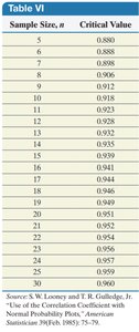
Sample Size, n	Critical Value
5	0.880
6	0.888
7	0.898
8	0.906
9	0.912
10	0.918
...	...
30	0.960

7.4 The Normal Approximation to the Binomial Probability Distribution

When certain conditions are met, the binomial distribution can be approximated by the normal distribution, simplifying probability calculations for large samples.

Criteria for Binomial Experiments

• The experiment consists of n independent trials.

• Each trial has two outcomes: success or failure.

• The probability of success (p) is constant for each trial.

Normal Approximation Conditions

• If $np(1-p) \geq 10$, the binomial distribution is approximately normal.

• Mean: $\mu = np$

• Standard deviation: $\sigma = \sqrt{np(1-p)}$

Example Applications

• For 100 flights with a 3.23% cancellation rate, check if $np(1-p) \geq 10$ to use the normal approximation.

• For 200 households with 8.5% buying gifts for dogs, calculate expected value, standard deviation, and probabilities using the normal approximation.

Additional info:

• Continuity correction is often applied when using the normal approximation for discrete distributions.