Chapter 9: Inferring Population Means – Confidence Intervals and Hypothesis Tests

Inferring Population Means

Introduction

This chapter focuses on statistical methods for making inferences about population means using sample data. The primary tools are confidence intervals and hypothesis tests, which allow us to estimate population parameters and test claims about them. The Central Limit Theorem (CLT) and the t-distribution are foundational concepts for these methods.

Sampling Distributions and the Central Limit Theorem

Sampling Distribution of the Mean

The sampling distribution of the mean is the probability distribution of all possible sample means from samples of a given size drawn from a population. It is described by its shape, center, and spread:

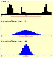
• Shape: As sample size increases, the sampling distribution approaches a normal distribution, regardless of the population's original shape (for n > 25).

• Center: The mean of the sampling distribution equals the population mean (μ).

• Spread: The standard deviation of the sampling distribution is called the standard error (SE).

Notation: μ = population mean, \( \bar{x} \) = sample mean, σ = population standard deviation, s = sample standard deviation.

Central Limit Theorem (CLT)

The Central Limit Theorem states that, for a sufficiently large sample size, the distribution of sample means will be approximately normal, regardless of the population's distribution. If the population is normal, the sample size does not matter.

• Conditions for CLT:

  • Random and independent sample

  • Large sample size (n ≥ 25, or population is normal)

  • Population at least 10 times larger than the sample (if sampling without replacement)

The standard error of the mean is given by:

$ SE = \frac{\sigma}{\sqrt{n}} $

If σ is unknown, use s (sample standard deviation):

$ SE = \frac{s}{\sqrt{n}} $

Visualizing the Effect of Sample Size

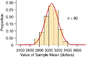
As sample size increases, the sampling distribution becomes more normal and the standard error decreases.

Examples of the Central Limit Theorem

• Weights of 10-Year-Old Boys: Given a normal population with mean 88.3 lbs and standard deviation 2.06 lbs, the probability that the sample mean for n = 30 exceeds 89 lbs can be found using the normal distribution.

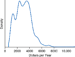
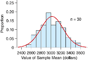
• Home Prices: For a skewed population, a large sample (n ≥ 25) allows use of the CLT to approximate probabilities for the sample mean.

The t-Distribution

Introduction to the t-Statistic

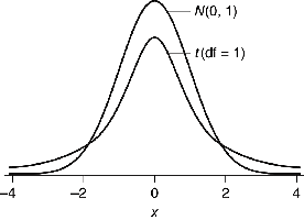
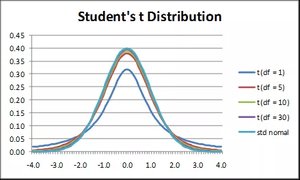
The t-distribution is used when the population standard deviation (σ) is unknown. It is similar to the normal distribution but has thicker tails, which accounts for the extra uncertainty from estimating σ with s. The shape depends on the degrees of freedom (df = n - 1).

• As sample size increases, the t-distribution approaches the normal distribution.

• Use the t-distribution for hypothesis tests and confidence intervals when σ is unknown.

Formula for the t-Statistic

$ t = \frac{\bar{x} - \mu_0}{\frac{s}{\sqrt{n}}} $

Where \( \bar{x} \) is the sample mean, \( \mu_0 \) is the hypothesized population mean, s is the sample standard deviation, and n is the sample size.

Confidence Intervals for a Population Mean

Constructing a Confidence Interval

A confidence interval provides a range of plausible values for the population mean. The general form is:

$ \bar{x} \pm t^* \left( \frac{s}{\sqrt{n}} \right) $

• \( t^* \) is the critical value from the t-distribution for the desired confidence level and degrees of freedom (df = n - 1).

• Conditions: random, independent sample; large sample size or normal population; large population if sampling without replacement.

Example: Highway Speeds

Given a sample mean speed of 63.3 mph, standard deviation 5.23 mph, and n = 30, the 95% confidence interval is calculated as follows:

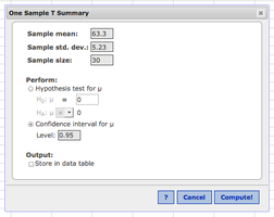
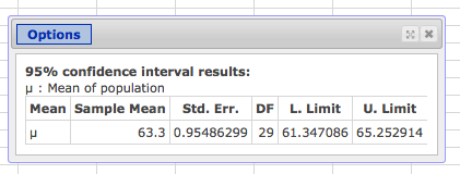
Interpretation: We are 95% confident that the mean speed of cars on the highway is between 61.35 and 65.25 mph.

Effect of Confidence Level and Sample Size

• Higher confidence level → wider interval (larger t*)

• Larger sample size → smaller standard error → narrower interval

Hypothesis Testing for a Population Mean

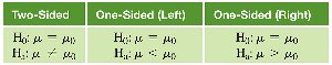
Four Steps for Hypothesis Testing

1. Hypothesize: State null (H0) and alternative (Ha) hypotheses.

2. Prepare: Check conditions, choose significance level (α), and select test statistic.

3. Compute: Calculate the test statistic and p-value.

4. Compare and Interpret: Compare p-value to α and draw a conclusion.

Example: Nursing Staff Experience

Given a sample mean of 18.37 years, standard deviation 11.12 years, n = 35, and a hypothesized mean of 14.3 years, a t-test is performed. If the p-value is less than α = 0.05, we reject H0 and conclude that the mean experience has increased.

Comparing Two Population Means

Independent vs. Dependent Samples

• Independent samples: Two separate groups (e.g., day vs. evening students).

• Dependent (matched pairs): Paired or repeated measurements (e.g., pre-test/post-test on the same individuals).

Confidence Interval for the Difference of Means (Independent Samples)

For two independent samples, the confidence interval for the difference in means is:

$ (\bar{x}_1 - \bar{x}_2) \pm t^* \cdot SE_{\text{difference}} $

Where:

$ SE_{\text{difference}} = \sqrt{ \frac{s_1^2}{n_1} + \frac{s_2^2}{n_2} } $

Hypothesis Test for the Difference of Means

Null hypothesis: $ H_0: \mu_1 = \mu_2 $ Alternative hypothesis: $ H_a: \mu_1 \neq \mu_2 $ (or one-sided)

Test statistic:

$ t = \frac{ (\bar{x}_1 - \bar{x}_2) - (\mu_1 - \mu_2)_{H_0} }{ SE_{\text{difference}} } $

Example: College Credits

Given summary statistics for day and evening students, a 95% confidence interval for the difference in mean credits is calculated. If the interval does not contain 0, there is a significant difference.

Matched Pairs (Dependent Samples)

For matched pairs, calculate the difference for each pair and analyze the differences as a single sample. Use a one-sample t-test or confidence interval for the mean difference.

Summary and Comparison of Methods

• Hypothesis tests and confidence intervals for means use similar calculations and conditions.

• For two-sided alternatives, confidence intervals and hypothesis tests yield the same conclusion.

• For one-sided alternatives, only hypothesis tests are appropriate.

• Do not "accept" the null hypothesis; only fail to reject it if evidence is insufficient.