Chi-Square Tests: Goodness-of-Fit, Independence, and Homogeneity

Chi-Square Tests for Categorical Data

Introduction to Chi-Square Tests

Chi-square tests are a family of statistical tests used to analyze categorical data. They are particularly useful for testing hypotheses about the distribution of categorical variables and the relationships between them. The three main types of chi-square tests are the goodness-of-fit test, the test for independence, and the test for homogeneity of proportions.

Goodness-of-Fit Test

Purpose and Overview

The goodness-of-fit test is used to determine whether the observed frequency distribution of a categorical variable matches an expected distribution. This test is commonly applied when comparing sample data to a known or hypothesized population distribution.

• Null Hypothesis (H0): The observed distribution matches the expected distribution.

• Alternative Hypothesis (H1): The observed distribution does not match the expected distribution.

Characteristics of the Chi-Square Distribution

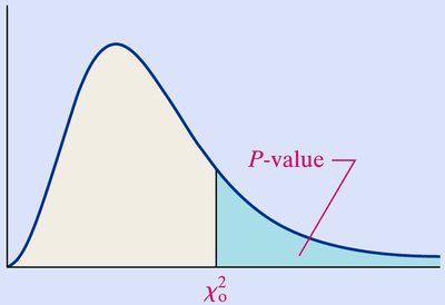
• Not symmetric; skewed right, especially for small degrees of freedom (d.f.).

• The shape depends on the degrees of freedom, becoming more symmetric as d.f. increases.

• All values are nonnegative (χ² ≥ 0).

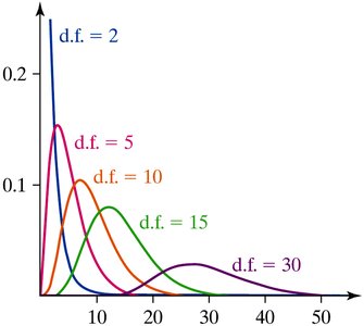
Calculating Expected Counts

Suppose there are n independent trials and k mutually exclusive categories. Let pi be the probability of the ith outcome. The expected count for each category is:

$E_i = n p_i \quad \text{for} \ i = 1, 2, \ldots, k$

• All expected counts should be at least 1, and no more than 20% should be less than 5.

Example: Expected Counts Calculation

A sociologist wants to know if the distribution of years grandparents care for grandchildren has changed since 2000. The 2000 distribution is:

Number of Years	Probability
Less than 1 year	0.228
1 or 2 years	0.239
3 or 4 years	0.176
5 or more years	0.357

For a sample of 1,000 grandparents, the expected counts are:

• Less than 1 year: $E = 1000 \times 0.228 = 228$

• 1 or 2 years: $E = 1000 \times 0.239 = 239$

• 3 or 4 years: $E = 1000 \times 0.176 = 176$

• 5 or more years: $E = 1000 \times 0.357 = 357$

Test Statistic for Goodness-of-Fit

The test statistic is calculated as:

$\chi^2 = \sum_{i=1}^{k} \frac{(O_i - E_i)^2}{E_i}$

where $O_i$ is the observed count and $E_i$ is the expected count for category $i$.

• The test statistic approximately follows a chi-square distribution with $k-1$ degrees of freedom.

Steps for Conducting a Goodness-of-Fit Test

1. State the hypotheses: $H_0$: The variable follows the specified distribution; $H_1$: It does not.

2. Choose a significance level ($\alpha$), e.g., 0.05.

3. Calculate expected counts and verify requirements.

4. Compute the test statistic using the formula above.

5. Determine the critical value from the chi-square table for $k-1$ degrees of freedom.

6. Compare the test statistic to the critical value (classical approach) or compute the P-value (P-value approach).

7. State the conclusion based on the comparison.

Critical Value and P-Value Approaches

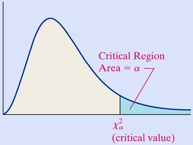
• Critical Value Approach: Reject $H_0$ if $\chi^2_0 > \chi^2_{\alpha}$ (critical value).

• P-Value Approach: Reject $H_0$ if P-value $< \alpha$.

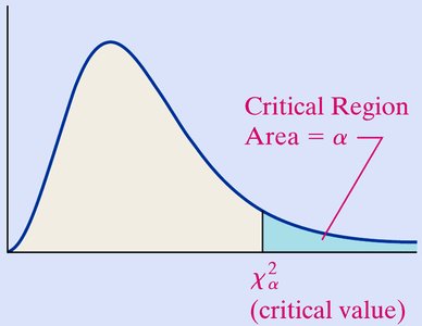
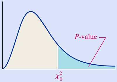
Worked Example: Goodness-of-Fit Test

Observed counts for the number of years grandparents care for grandchildren:

Number of Years	Frequency
Less than 1 year	252
1 or 2 years	255
3 or 4 years	162
5 or more years	331

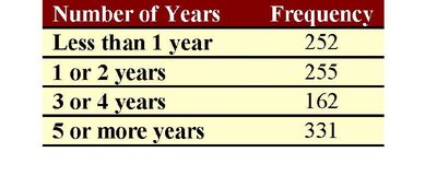
Test statistic: $\chi^2_0 = 6.605$; Critical value at $\alpha = 0.05$ and 3 d.f.: $7.815$.

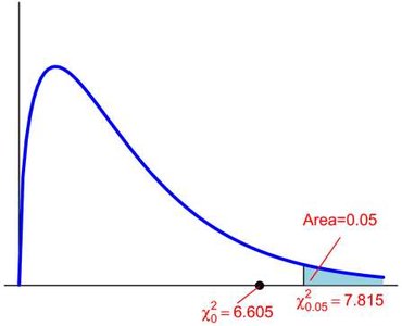
Since $6.605 < 7.815$, we fail to reject $H_0$. The P-value ($\approx 0.09$) is also greater than $0.05$.

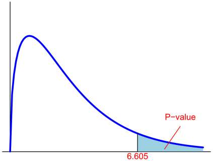
Conclusion: There is insufficient evidence to conclude that the distribution has changed.

Chi-Square Test for Independence

Purpose and Overview

The chi-square test for independence is used to determine whether two categorical variables are associated (dependent) or not (independent). Data are organized in a contingency table.

• Null Hypothesis (H0): The variables are independent.

• Alternative Hypothesis (H1): The variables are dependent.

Calculating Expected Counts in Contingency Tables

For a cell in row $i$ and column $j$:

$E_{ij} = \frac{(\text{row total}) \times (\text{column total})}{\text{table total}}$

Example: Expected Counts Calculation

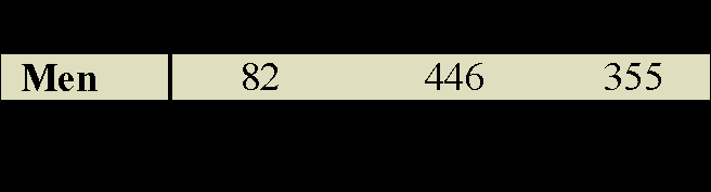
	Money	Health	Love	Row Totals
Men	82	446	355	883
Women	46	574	273	893
Column Totals	128	1020	628	1776

Test Statistic for Independence

The test statistic is:

$\chi^2 = \sum_{i=1}^{r} \sum_{j=1}^{c} \frac{(O_{ij} - E_{ij})^2}{E_{ij}}$

where $r$ is the number of rows and $c$ is the number of columns. The degrees of freedom are $(r-1)(c-1)$.

Steps for Conducting a Test for Independence

1. State the hypotheses: $H_0$: Variables are independent; $H_1$: Variables are dependent.

2. Choose a significance level ($\alpha$).

3. Calculate expected counts and verify requirements.

4. Compute the test statistic.

5. Determine the critical value or P-value.

6. Draw a conclusion.

Worked Example: Test for Independence

Observed and expected counts for the poll:

	Money	Health	Love
Men	82 (63.58)	446 (507.05)	355 (312.22)
Women	46 (64.29)	574 (512.91)	273 (315.77)

Test statistic: $\chi^2_0 \approx 36.82$; Critical value at $\alpha = 0.05$ and 2 d.f.: $5.99$.

Since $36.82 > 5.99$, we reject $H_0$. The P-value is approximately 0 (less than $0.05$).

Conclusion: There is sufficient evidence to conclude that gender and response are dependent.

Conditional Distributions and Bar Graphs

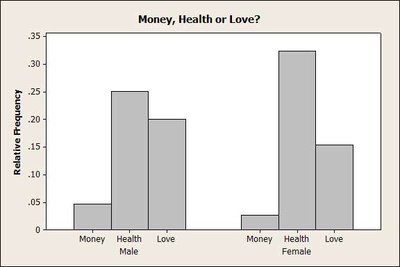
Conditional distributions show the relative frequency of each response by gender:

	Money	Health	Love
Men	0.0929	0.5051	0.4020
Women	0.0515	0.6428	0.3057

Chi-Square Test for Homogeneity of Proportions

Purpose and Overview

The chi-square test for homogeneity of proportions is used to test whether different populations have the same proportion of individuals with a certain characteristic. The procedure is identical to the test for independence, but the context involves comparing populations rather than variables within a single population.

• Null Hypothesis (H0): All population proportions are equal.

• Alternative Hypothesis (H1): At least one proportion is different.

Worked Example: Test for Homogeneity

	1992	2002	2008
Yes	418 (475.554)	479 (475.554)	525 (470.892)
No	602 (544.446)	541 (544.446)	485 (539.108)

Test statistic: $\chi^2_0 \approx 24.74$; Critical value at $\alpha = 0.01$ and 2 d.f.: $9.210$.

Since $24.74 > 9.210$, we reject $H_0$. The P-value is approximately 0 (less than $0.01$).

Conclusion: There is sufficient evidence to conclude that the proportion of individuals who believe teaching is a prestigious career differs among the years.

Summary Table: Chi-Square Test Types

Test	Purpose	Data Structure	Degrees of Freedom
Goodness-of-Fit	Compare observed to expected distribution	One categorical variable, k categories	k - 1
Independence	Test association between two variables	Contingency table (r x c)	(r - 1)(c - 1)
Homogeneity	Compare proportions across populations	Contingency table (r x c)	(r - 1)(c - 1)