Comparing Two Groups: Means, Proportions, and Dependent Samples in Statistical Inference

Comparing Two Groups in Statistical Inference

Introduction

Statistical inference often involves comparing two groups to determine if there is a significant difference between them. This can involve comparing means or proportions, and the groups may be independent or dependent (matched pairs). The following notes summarize key concepts, methods, and examples for comparing two groups, including the use of permutation tests when assumptions for traditional tests are not met.

Comparing Two Independent Means

Confidence Intervals and Hypothesis Tests

When comparing the means of two independent groups, we estimate the difference between the population means (μ1 - μ2) using the difference in sample means (\( \bar{x}_1 - \bar{x}_2 \)).

• Standard Error: \( \sqrt{ \frac{s_1^2}{n_1} + \frac{s_2^2}{n_2} } \)

• Confidence Interval: \( (\bar{x}_1 - \bar{x}_2) \pm t^* \sqrt{ \frac{s_1^2}{n_1} + \frac{s_2^2}{n_2} } \)

• Test Statistic: \( t = \frac{ (\bar{x}_1 - \bar{x}_2) - 0 }{ \sqrt{ \frac{s_1^2}{n_1} + \frac{s_2^2}{n_2} } } \)

• Assumptions: Independent random samples, approximately normal distributions (especially important for small samples).

Interpretation: If the confidence interval for the difference does not include zero, there is evidence of a significant difference between the groups.

Example: Comparing Email Hours per Week by Age Group

Suppose we want to compare the average number of hours spent on email per week between 18-year-olds and 30-year-olds. The data are summarized below:

• 18-year-olds: n = 9, mean = 5.33, SD = 9.7

• 30-year-olds: n = 10, mean = 6.10, SD = 3.0

Initial analysis (with outlier):

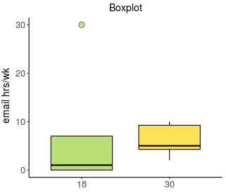
The boxplot shows an outlier in the 18-year-old group, which may affect the results.

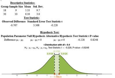
The test statistic is -0.228 with a p-value of 0.8248, indicating no significant difference in mean email hours per week between the two age groups when the outlier is included.

After removing the outlier:

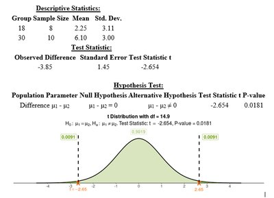
The test statistic becomes -2.654 with a p-value of 0.0181, suggesting a significant difference. However, since the conclusion depends heavily on one observation, and the sample size is small, caution is warranted. The assumption of normality may not be satisfied, so results should be interpreted carefully.

Comparing Means from Dependent Samples (Matched Pairs)

Paired t-Test

When the same subjects are measured twice (e.g., before and after treatment), or when pairs are matched, we analyze the differences within each pair.

• Difference for each pair: \( d_i = x_{i,1} - x_{i,2} \)

• Mean and SD of differences: \( \bar{d}, s_d \)

• Standard Error: \( \frac{s_d}{\sqrt{n}} \)

• Confidence Interval: \( \bar{d} \pm t^* \frac{s_d}{\sqrt{n}} \)

• Test Statistic: \( t = \frac{\bar{d} - 0}{s_d / \sqrt{n}} \)

• Assumptions: Random sample of differences, differences are approximately normally distributed (especially important for small n).

Example: Effect of Yoga on Running Times

Ten runners measured their 5K times before and after a yoga program. The differences (before - after) are plotted below:

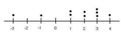
The dotplot shows no major outliers, so t-procedures are reasonable. The 95% confidence interval for the mean difference is (-0.116, 2.916) minutes. The paired t-test yields a p-value between 0.025 and 0.05, suggesting some evidence that yoga improves running times, but the CI includes zero, so results are not conclusive at the 0.05 level.

Permutation Tests for Comparing Two Groups

When to Use Permutation Tests

If the assumptions of normality are not met for the two-sample t-test (e.g., small sample sizes, skewed data, or outliers), permutation tests provide a nonparametric alternative. They do not rely on the sampling distributions of the test statistics but instead use the observed data to generate a reference distribution by randomly reassigning group labels.

• Assumptions: Quantitative response variable, independent random samples or randomized experiments.

• Test Statistic: Difference in sample means (or medians).

• P-value: Proportion of permutations with a test statistic as extreme or more extreme than observed.

Example: Comparing Number of Text Messages

In-state and out-of-state students were compared on the number of text messages received in 24 hours. The permutation test sampling distribution is shown below:

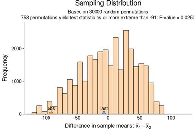
With a p-value of 0.0253, there is fairly strong evidence that in-state students receive fewer text messages than out-of-state students. The permutation test is appropriate here due to small sample sizes and possible skewness in the data.

Summary Table: Choosing the Appropriate Test

Situation	Test	Key Assumptions
Compare means, independent groups	Two-sample t-test	Normality, independent random samples
Compare means, matched pairs	Paired t-test	Normality of differences, random sample
Compare means, small/non-normal samples	Permutation test	Random assignment or sampling

Key Points

• Always check assumptions before choosing a test.

• Outliers and small sample sizes can greatly affect results; consider nonparametric alternatives when needed.

• Permutation tests are flexible and robust when traditional assumptions are not met.