Confidence Intervals for Means: The t-Distribution and Its Applications

Confidence Intervals for Means

Introduction to Confidence Intervals

A confidence interval is a range of values, derived from sample statistics, that is likely to contain the value of an unknown population parameter. In the context of means, confidence intervals estimate the population mean based on sample data.

• Population Parameter (μ): The true mean of the population.

• Sample Statistic (\( \bar{y} \)): The mean calculated from the sample.

• Confidence Level: The probability that the interval contains the population parameter (commonly 90%, 95%, or 99%).

Confidence intervals are interpreted as the range in which we are reasonably certain the population mean lies, given our sample data.

Sampling Distribution and the Central Limit Theorem (CLT)

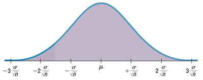
The Central Limit Theorem states that, for a sufficiently large sample size, the sampling distribution of the sample mean will be approximately normal, regardless of the population's distribution. This allows us to use normal or t-distributions to construct confidence intervals for means.

• Sampling Distribution: \( \bar{x} \sim N(\mu, \frac{\sigma}{\sqrt{n}}) \)

• Standard Error (SE): \( SE = \frac{s}{\sqrt{n}} \), where s is the sample standard deviation.

Conditions for Constructing Confidence Intervals

Before constructing a confidence interval for the mean, certain conditions must be met:

• Independence: Data should be mutually independent.

• Randomization: Data should come from a random sample or randomized experiment.

• 10% Condition: Sample size should be less than 10% of the population (\( n < 0.1N \)).

• Nearly Normal Condition: For small samples, data should be nearly normal. For larger samples (\( n > 40 \)), t-methods are robust to moderate skewness.

Estimating the Population Mean: z vs. t

When the population standard deviation (\( \sigma \)) is known, the normal (z) distribution is used. However, in practice, \( \sigma \) is rarely known, so the sample standard deviation (s) is used, introducing extra variability. This is accounted for by using the Student's t-distribution.

• z-interval: Use when \( \sigma \) is known.

• t-interval: Use when \( \sigma \) is unknown and estimated by s.

The Student's t-Distribution

Origin and Properties

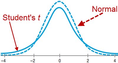
The Student's t-distribution was developed by William Sealy Gosset ("Student") to address the increased variability when estimating \( \sigma \) with s, especially for small samples. The t-distribution is bell-shaped, symmetric, and unimodal, but has heavier tails than the normal distribution.

• Degrees of Freedom (df): \( df = n - 1 \), where n is the sample size.

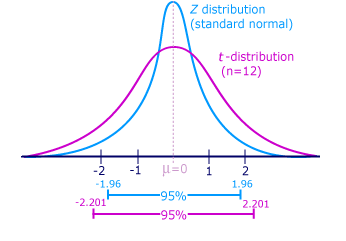
• As df increases, the t-distribution approaches the normal distribution.

• For small df, the t-distribution has fatter tails, reflecting greater uncertainty.

Formula for a One-Sample t-Interval for the Mean

When assumptions are met, the confidence interval for the mean is:

• \( \bar{y} \pm t^*_{n-1} \cdot SE(\bar{y}) \)

• Where \( SE(\bar{y}) = \frac{s}{\sqrt{n}} \)

• \( t^*_{n-1} \) is the critical value from the t-distribution with \( n-1 \) degrees of freedom for the desired confidence level.

As sample size increases, \( s \) becomes a better estimate of \( \sigma \), and the t-distribution approaches the normal distribution.

Example: Confidence Interval for Mean Contaminant Concentration

Suppose a study of contaminant concentrations in farm-raised salmon yields:

• n = 150

• \( \bar{y} = 0.0913 \) ppm

• s = 0.0495 ppm

• df = 149

• 95% CI: \( 0.0913 \pm 1.976 \times 0.0040 = (0.0834, 0.0992) \)

Interpretation: We are 95% confident that the mean contaminant concentration in farm-raised salmon is between 0.0834 and 0.0992 ppm.

Checking Assumptions and Conditions: Examples

• Randomization: Data should be from a random or representative sample.

• Nearly Normal: For n = 30, check histogram for unimodality and symmetry.

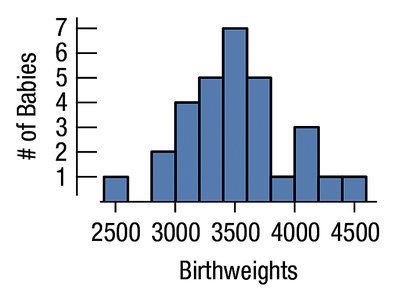
For n = 30 babies, the histogram is unimodal and symmetric, so t-methods are appropriate.

Mechanics of Calculating a t-Interval

• \( \bar{y} = 3498.7 \) grams, s = 434.2 grams, n = 30

• \( SE = \frac{434.2}{\sqrt{30}} \approx 79.27 \) grams

• \( t^*_{29} = 1.699 \) for 90% confidence

• Margin of Error: \( 1.699 \times 79.27 = 134.68 \) grams

• 90% CI: \( 3498.7 \pm 134.68 = (3364.0, 3633.4) \) grams

Interpretation: We are 90% confident that the true mean birthweight of U.S. babies born in 1998 is between 3364.0 and 3633.4 grams.

Summary Table: z vs. t Confidence Intervals

Situation	Distribution	Formula
Population SD known	Normal (z)	\( \bar{y} \pm z^* \frac{\sigma}{\sqrt{n}} \)
Population SD unknown	t-distribution	\( \bar{y} \pm t^*_{n-1} \frac{s}{\sqrt{n}} \)

Interpreting Confidence Intervals

A correct interpretation of a confidence interval for a mean is: "We are [confidence level]% confident that the interval from [lower bound] to [upper bound] contains the true population mean."

Practice Problems: Identifying the Correct Formula

Scenario	Correct Formula
Sample mean = 12.32, s = 1.88, n = 10, 95% CI	\( 12.32 \pm t^*_{9} \frac{1.88}{\sqrt{10}} \)
Sample mean = 12.5, s = 0.5, n = 10, 95% CI	\( 12.5 \pm t^*_{9} \frac{0.5}{\sqrt{10}} \)

Key Properties of the t-Distribution

• Unimodal and symmetric (mound-shaped)

• Has heavier tails than the normal distribution (more spread for small n)

• As degrees of freedom increase, the t-distribution approaches the normal distribution and variance decreases