Confidence Intervals for Proportions and Means

Confidence Intervals for Proportions and Means

Point Estimators and Interval Estimates

In statistics, we use sample statistics as point estimators to estimate unknown population parameters. For example, the sample mean (\( \bar{y} \)) estimates the population mean (\( \mu \)), and the sample proportion (\( \hat{p} \)) estimates the population proportion (\( p \)). However, these statistics vary from sample to sample, so we use interval estimates to express the uncertainty in our estimates.

• Unbiased Estimator: The long-run average of the estimator equals the parameter being estimated.

• Reliability: The statistic from a single sample should be close to the true parameter; reliability is expressed as confidence.

• Consistency: As sample size increases, the estimator becomes more accurate.

Confidence Intervals: Definition and Purpose

A confidence interval is an interval within which we expect the true value of a population parameter to lie, based on sample data. The most common types are for the mean, median, proportion, standard deviation, and variance. This chapter focuses on confidence intervals for population proportions.

Confidence Intervals for a Population Proportion

Sampling Distribution and Standard Error

The sampling distribution of the sample proportion (\( \hat{p} \)) is approximately normal, centered at \( p \), with standard deviation:

$\sigma_{\hat{p}} = \sqrt{\frac{p(1-p)}{n}}$

Since p is unknown, we estimate the standard deviation using the sample proportion, calling it the standard error (SE):

$SE(\hat{p}) = \sqrt{\frac{\hat{p}(1-\hat{p})}{n}}$

Constructing a Confidence Interval

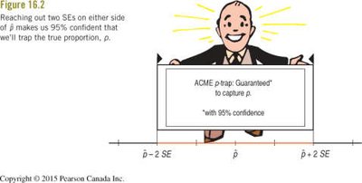
By the 68-95-99.7% Rule, about 95% of all samples will have \( \hat{p} \) within 2 SEs of p. Thus, a 95% confidence interval for p is:

$\hat{p} \pm 2 \times SE(\hat{p})$

Confidence and the Normal Distribution

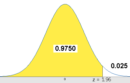
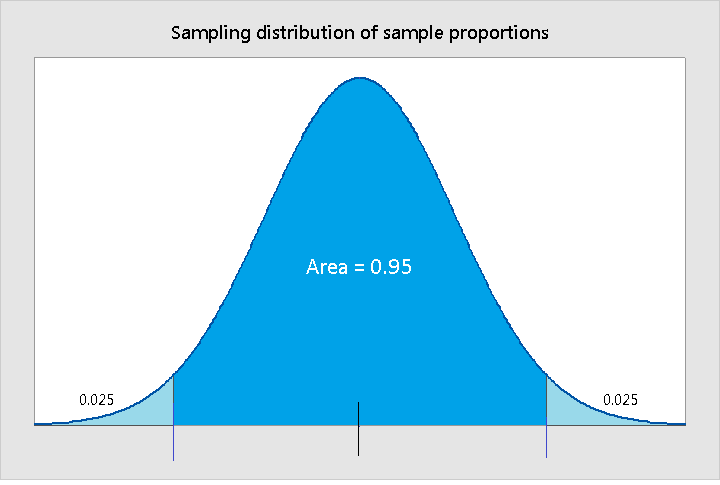
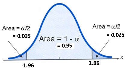
More precisely, 95% of the area under the normal curve lies between z-scores of -1.96 and +1.96. Thus, the 95% confidence interval is:

$\hat{p} \pm 1.96 \times SE(\hat{p})$

Interpreting Confidence Intervals

"95% confidence" means that if we were to take many samples and build a confidence interval from each, about 95% of those intervals would contain the true population proportion p. For any single interval, we say we are 95% confident that it contains p.

Critical Values for Different Confidence Levels

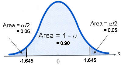
The critical value z\alpha/2 depends on the desired confidence level:

• For 90% confidence: z\alpha/2 = 1.645

• For 95% confidence: z\alpha/2 = 1.96

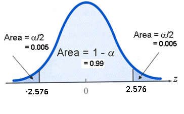
• For 99% confidence: z\alpha/2 = 2.576

Confidence Level	Risk (\( \alpha \))	Critical Value (\( z_{\alpha/2} \))
90%	0.10	±1.645
95%	0.05	±1.96
99%	0.01	±2.576

Assumptions and Conditions for Proportion Intervals

Before constructing a confidence interval for a proportion, check these conditions:

• Independence Assumption: The sampled values must be independent.

• Randomization Condition: Data must be from a random sample or randomized experiment.

• 10% Condition: Sample size should be no more than 10% of the population.

• Success/Failure Condition: Expect at least 10 successes and 10 failures: np ≥ 10 and n(1-p) ≥ 10.

Formula: One-Proportion z-Interval

When the above conditions are met, the confidence interval for a population proportion is:

$\hat{p} \pm z_{\alpha/2} \sqrt{\frac{\hat{p}(1-\hat{p})}{n}}$

• \( \hat{p} \): sample proportion

• n: sample size

• z\alpha/2: critical value for desired confidence level

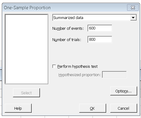
Example: Effectiveness of a Flu Shot

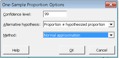
Suppose 800 students are randomly selected and given a flu shot; 600 do not get the flu. Find a 99% confidence interval for the effectiveness of the flu shot.

• Sample size: n = 800

• Sample proportion: \( \hat{p} = 600/800 = 0.75 \)

• Critical value for 99%: 2.576

• Standard error: $SE = \sqrt{\frac{0.75 \times 0.25}{800}} = 0.0153$

• Confidence interval: $0.75 \pm 2.576 \times 0.0153 = 0.75 \pm 0.04 = [0.71, 0.79]$

Interpretation: We are 99% confident that the true effectiveness of the flu shot is between 71% and 79%.

Margin of Error (ME)

The margin of error is the amount added and subtracted from the point estimate to form the confidence interval:

$ME = z_{\alpha/2} \times SE(\hat{p})$

Higher confidence levels increase the margin of error, making the interval wider. Larger sample sizes decrease the margin of error, making the interval narrower.

Choosing Sample Size for Proportions

To estimate a population proportion within a desired margin of error (ME) and confidence level, use:

$n = \frac{z_{\alpha/2}^2 \hat{p}(1-\hat{p})}{ME^2}$

If no prior estimate for \( \hat{p} \) is available, use 0.5 for a conservative estimate.

Plus Four Confidence Interval for Small Samples

If the Success/Failure Condition fails, add two successes and two failures to the data:

$\tilde{p} = \frac{y + 2}{n + 4}$

Then use \( \tilde{p} \) in the confidence interval formula. This adjustment improves performance for small samples or proportions near 0 or 1.

Confidence Intervals for Population Means (Large Samples)

The Central Limit Theorem (CLT)

The CLT states that for large samples, the sampling distribution of the sample mean (\( \bar{y} \)) is approximately normal, regardless of the population's distribution. The mean is \( \mu \) and the standard deviation is \( \sigma/\sqrt{n} \).

If \( \sigma \) is unknown and n ≥ 60, use the sample standard deviation s as an estimate.

Formula: Confidence Interval for a Mean (z-interval)

$\bar{y} \pm z_{\alpha/2} \frac{s}{\sqrt{n}}$

• \( \bar{y} \): sample mean

• s: sample standard deviation

• n: sample size

• z\alpha/2: critical value for desired confidence level

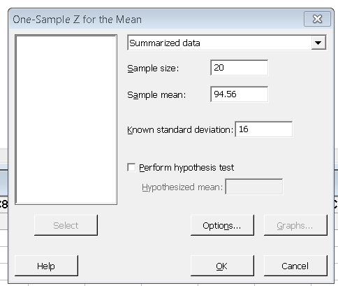
Example: IQ Scores

Suppose 20 people are sampled, mean IQ = 94.56, population standard deviation = 16. Find a 95% confidence interval for the mean IQ.

• Sample mean: 94.56

• Standard deviation: 16

• Sample size: 20

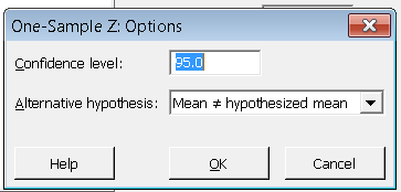
• Critical value for 95%: 1.96

• Standard error: $SE = 16/\sqrt{20} = 3.58$

• Confidence interval: $94.56 \pm 1.96 \times 3.58 = 94.56 \pm 7.01 = [87.55, 101.57]$

Choosing Sample Size for Means

To estimate a population mean within a desired margin of error (ME) and confidence level, use:

$n = \frac{z_{\alpha/2}^2 \sigma^2}{ME^2}$

If \( \sigma \) is unknown, use the sample standard deviation from a previous study or estimate using the range divided by 4.

What Can Go Wrong?

• Do not misinterpret the interval: it is the parameter that is fixed, not the interval.

• Do not claim that other samples will give the same interval.

• Do not be certain about the parameter; confidence intervals express uncertainty.

• Check all assumptions and conditions before using the formulas.

• Margin of error too large? Increase sample size or accept less confidence.

Summary Table: Confidence Intervals for Proportions and Means

Parameter	Confidence Interval Formula	Conditions
Proportion (p)	$\hat{p} \pm z_{\alpha/2} \sqrt{\frac{\hat{p}(1-\hat{p})}{n}}$	Random sample, independence, 10% condition, success/failure condition
Mean (\mu)	$\bar{y} \pm z_{\alpha/2} \frac{s}{\sqrt{n}}$	Random sample, n ≥ 60 if \sigma unknown, normality if \sigma unknown

Key Takeaways

• Confidence intervals provide a range of plausible values for population parameters.

• Higher confidence means wider intervals; larger samples mean narrower intervals.

• Always check assumptions before interpreting results.