Contingency Tables, Association, and Simpson’s Paradox in Introductory Statistics

Describing the Relation Between Two Variables

Contingency Tables and Association

Contingency tables, also known as two-way tables, are used to summarize the relationship between two categorical variables. They allow us to analyze how the distribution of one variable may depend on the value of another variable. This section covers how to compute marginal and conditional distributions, identify associations, and understand Simpson’s Paradox.

Contingency Tables: Structure and Terminology

• Contingency Table (Two-Way Table): A table that displays the frequency distribution of variables that are categorical. Each cell in the table shows the count for a specific combination of categories.

• Row Variable: The variable whose categories label the rows (e.g., grade received).

• Column Variable: The variable whose categories label the columns (e.g., delivery method).

• Cell: Each box inside the table, representing the count for a specific combination of row and column categories.

Marginal Distributions

The marginal distribution of a variable is the frequency or relative frequency distribution of either the row or column variable in a contingency table. Marginal distributions help us understand the overall distribution of each variable, ignoring the other variable.

• Frequency Marginal Distribution: The total counts for each category of a variable, found by summing across rows or columns.

• Relative Frequency Marginal Distribution: The proportion of the total for each category, calculated by dividing the frequency by the overall total.

• Example: In a study comparing traditional, online, and hybrid statistics courses, the marginal distribution for grades shows the total number of students earning each grade, regardless of delivery method.

Conditional Distributions and Association

A conditional distribution lists the relative frequencies of categories of the response variable, given a specific value of the explanatory variable. Conditional distributions are used to identify associations between categorical variables.

• Conditional Distribution: For each value of the explanatory variable, calculate the relative frequency of each category of the response variable.

• Association: If the conditional distributions differ across categories of the explanatory variable, there is evidence of an association between the variables.

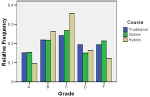
• Example: Students in a hybrid statistics course are more likely to pass (earn grades A, B, or C) compared to those in traditional or online courses, indicating an association between delivery method and grade earned.

Visualizing Conditional Distributions

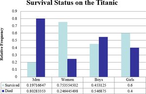
Bar graphs are commonly used to display conditional distributions, making it easier to compare the relative frequencies across categories.

• Example: The bar graph below shows the conditional distribution of survival status by demographic group (men, women, boys, girls) among Titanic passengers.

Simpson’s Paradox

Simpson’s Paradox occurs when an association between two variables reverses or disappears when a third variable (a lurking variable) is introduced into the analysis. This paradox highlights the importance of considering all relevant variables when interpreting data.

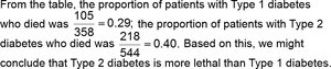
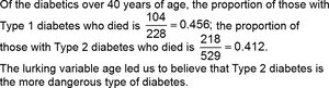
• Example: In a study of diabetes patients, the overall data suggested that Type 2 diabetes was more lethal than Type 1 diabetes. However, when the data were separated by age group, the association reversed, showing that Type 1 diabetes was more lethal among older patients, and there was no difference among younger patients.

• Mathematical Illustration:

Overall death rates:

• Type 1: $\frac{105}{358} = 0.29$

• Type 2: $\frac{218}{544} = 0.40$

Among patients 40 years or younger:

• Type 1: $\frac{1}{130} = 0.008$

• Type 2: $\frac{0}{15} = 0$

Among patients over 40 years:

• Type 1: $\frac{104}{228} = 0.456$

• Type 2: $\frac{218}{529} = 0.412$

This example demonstrates how a lurking variable (age) can change the interpretation of the data.

Summary Table: Key Concepts in Contingency Tables and Association

Concept	Definition	Example
Contingency Table	Table showing frequency distribution for two categorical variables	Grades by course delivery method
Marginal Distribution	Distribution of a single variable, summing over the other variable	Total students earning each grade
Conditional Distribution	Distribution of one variable for a fixed value of the other variable	Grade distribution for each delivery method
Association	Exists if conditional distributions differ across categories	Hybrid students more likely to pass
Simpson’s Paradox	Association reverses/disappears when a third variable is considered	Diabetes lethality by type and age