Correlation and Linear Regression: Study Notes for Introductory Statistics

Correlation and Regression

Overview

This chapter introduces the concepts of correlation and linear regression, which are fundamental tools in statistics for analyzing relationships between two quantitative variables. The focus is on understanding how to measure the strength of association and how to model the relationship using a regression line.

Section 9.1: Correlation

Definition and Purpose

Correlation measures the strength and direction of the linear relationship between two variables, typically denoted as x (independent variable) and y (dependent variable).

• Positive correlation: As x increases, y tends to increase.

• Negative correlation: As x increases, y tends to decrease.

• No correlation: No consistent relationship between x and y.

Correlation coefficient (r): A numerical value between -1 and 1 that quantifies the strength and direction of the linear relationship.

• r = 1: Perfect positive linear correlation

• r = -1: Perfect negative linear correlation

• r = 0: No linear correlation

Significance: Before performing regression analysis, it is important to verify that the correlation between the variables is statistically significant.

Section 9.2: Linear Regression

Regression Line (Line of Best Fit)

Once a significant linear correlation is established, the next step is to determine the equation of the regression line, which models the relationship between x and y. The regression line is the line for which the sum of the squares of the residuals is minimized.

• Regression line equation: $\hat{y} = mx + b$

• m: Slope of the line, representing the change in y for each unit increase in x

• b: y-intercept, representing the predicted value of y when x = 0

Predicted y-value: The value of y estimated from the regression equation for a given x.

Residuals

Residuals are the differences between the observed y-values and the predicted y-values for each data point. They are used to assess the accuracy of the regression model.

• For each data point, $d_i = \text{observed y-value} - \text{predicted y-value}$

• Residuals can be positive, negative, or zero.

• The regression line minimizes the sum of the squares of these residuals.

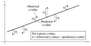
Finding the Regression Equation

Technology tools such as Excel, Minitab, and TI-84 calculators can be used to compute the regression equation efficiently. The process involves inputting the data and using built-in functions to obtain the slope and y-intercept.

• Excel: Use the SLOPE and INTERCEPT functions to calculate the regression coefficients.

• Minitab: Provides regression analysis output, including coefficients, standard errors, t-values, and p-values.

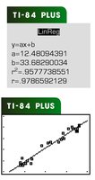
• TI-84 Plus: Computes the regression equation and displays the line of best fit along with the correlation coefficient ($r^2$).

Example: Old Faithful geyser data is used to illustrate the calculation of the regression line.

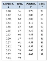
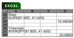
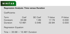
Interpreting the Regression Equation

The regression equation can be used to predict y-values for given x-values. For example, if the regression equation for gross domestic product (GDP) and carbon dioxide emissions is $\hat{y} = 199.535x + 56.036$, then for a GDP of $1.2$ trillion dollars:

• $\hat{y} = 199.535 \times 1.2 + 56.036 = 295.478$ (million metric tons)

Similarly, predictions can be made for other values of x.

Key Steps in Linear Regression Analysis

1. Verify that the correlation between x and y is significant.

2. Use technology or formulas to find the regression line equation.

3. Interpret the slope and y-intercept in the context of the data.

4. Use the regression equation to predict y-values for given x-values.

5. Analyze residuals to assess the fit of the model.

Summary Table: Regression Analysis Outputs

Tool	Slope	Y-intercept	Additional Outputs
Excel	12.48094	33.6829	Functions: SLOPE, INTERCEPT
Minitab	12.481	33.68	SE Coef, T-Value, P-Value
TI-84 Plus	12.48094391	33.6829034	$r^2$ value, scatterplot

Additional info:

Linear regression is a foundational technique in statistics, widely used in fields such as economics, biology, engineering, and social sciences to model and predict relationships between variables. Understanding how to interpret the slope and y-intercept is crucial for meaningful analysis. Residual analysis helps ensure the model's validity and detect potential outliers or non-linear patterns.