Chapter 9- Correlation and Regression: Concepts, Calculations, and Applications

Correlation and Regression

Introduction to Correlation and Regression

Correlation and regression are fundamental statistical techniques used to examine and model the relationship between two or more variables. Correlation quantifies the strength and direction of a linear relationship, while regression allows for prediction and explanation of one variable based on another.

Correlation

Definition and Purpose

• Correlation measures the degree to which two variables move together.

• The correlation coefficient (denoted as r for samples, \rho for populations) quantifies the strength and direction of a linear relationship.

• Values of r range from -1 to +1:

  • r = 1: Perfect positive linear correlation

  • r = -1: Perfect negative linear correlation

  • r = 0: No linear correlation

• Correlation does not imply causation.

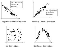
Types of Correlation

• Positive Linear Correlation: As one variable increases, the other tends to increase.

• Negative Linear Correlation: As one variable increases, the other tends to decrease.

• No Correlation: No discernible linear relationship between variables.

• Nonlinear Correlation: Variables are related, but not in a linear fashion.

Calculating the Correlation Coefficient

• The most common measure is the Pearson Product-Moment Correlation Coefficient (PPMCC).

• Sample correlation coefficient formula (definitional):

$r = \frac{\sum (x_i - \bar{x})(y_i - \bar{y})}{\sqrt{\sum (x_i - \bar{x})^2 \sum (y_i - \bar{y})^2}}$

• Computational formula (for paired data):

$r = \frac{n\sum xy - \sum x \sum y}{\sqrt{[n\sum x^2 - (\sum x)^2][n\sum y^2 - (\sum y)^2]}}$

• n is the number of paired observations.

• r estimates the population correlation coefficient \rho.

Assumptions of Pearson Correlation

• Variables are measured on an interval or ratio scale.

• Data are normally distributed.

• Relationship between variables is linear.

• If assumptions are violated or data are ordinal, use Spearman’s \( \rho \) instead.

Interpreting the Correlation Coefficient

• Strength: The closer |r| is to 1, the stronger the linear relationship.

• Direction: Positive values indicate direct relationships; negative values indicate inverse relationships.

• Coefficient of Determination (r2): Proportion of variance in y explained by x.

$r^2 = (\text{correlation coefficient})^2$

• For example, if r = 0.79, then r2 = 0.6241, meaning 62.41% of the variance in y is explained by x.

Testing the Significance of Correlation

• Null hypothesis: H0: \( \rho = 0 \) (no correlation)

• Alternative hypothesis: Ha: \( \rho \neq 0 \) (significant correlation)

• Test statistic:

$t = \frac{r\sqrt{n-2}}{\sqrt{1-r^2}}$

• Degrees of freedom: n – 2

• Compare calculated t to critical t-value or use p-value from statistical software.

Correlation and Causation

• Correlation does not imply causation.

• To infer causation, additional criteria must be met (e.g., temporal precedence, ruling out confounders).

• Spurious correlations can occur due to shared underlying causes.

Regression

Introduction to Regression

Regression analysis is used to predict the value of a dependent variable (y) based on the value of at least one independent variable (x). Simple linear regression involves one predictor; multiple regression involves two or more predictors.

Simple Linear Regression Model

• The equation for a straight line is:

$y = mx + b$

• In statistics, the regression equation is:

$\hat{y} = a + bx$

• \( \hat{y} \): Predicted value of y

• a: Intercept (value of y when x = 0)

• b: Slope (expected change in y for a one-unit increase in x)

Calculating Regression Coefficients

• The slope (b) can be calculated as:

$b = r \frac{s_y}{s_x}$

• The intercept (a) is:

$a = \bar{y} - b\bar{x}$

• Where \( \bar{x} \) and \( \bar{y} \) are the means of x and y, and \( s_x \), \( s_y \) are their standard deviations.

Standardized Regression Coefficient (Beta)

• When variables are standardized, the regression coefficient is called beta (\( \beta \)).

• \( \beta \) represents the expected change in y (in standard deviation units) for a one standard deviation change in x.

• In simple regression, \( \beta = r \).

Interpreting Regression Output

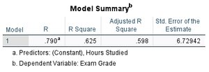
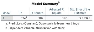
• Model Summary Table: Provides R, R2, adjusted R2, and standard error of the estimate.

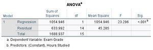
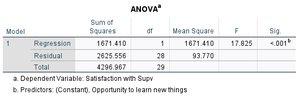
• ANOVA Table: Tests overall model significance (F-test).

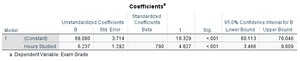
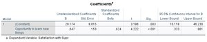
• Coefficients Table: Shows estimates for intercept and slope, their standard errors, t-values, and significance.

Example: Predicting Exam Grades from Study Hours

• Suppose r = 0.790 between hours studied (x) and exam grade (y).

• Regression equation: \( \hat{y} = 68.08 + 6.237x \)

• Interpretation: For each additional hour studied, exam grade increases by about 6.24 points.

• R2 = 0.625: 62.5% of the variance in exam grades is explained by hours studied.

Significance Testing in Regression

• Test whether slope (b) is significantly different from zero (H0: b = 0).

• Test whether intercept (a) is significantly different from zero (less common in social sciences).

• Test whether R2 is significantly different from zero.

Multiple Regression

• Involves two or more predictors.

• Allows assessment of the unique contribution of each predictor to the outcome variable.

• Example: Predicting PTSD among first responders using trauma exposure, organizational support, commitment, and tenure.

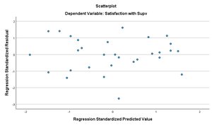
SPSS Output Interpretation: Satisfaction with Supervisor Example

• Dependent variable: Satisfaction with supervisor

• Predictor: Opportunity to learn new things

• R = 0.624, R2 = 0.389: 38.9% of variance in satisfaction explained by opportunity to learn.

• F(1,28) = 17.825, p < .001: Model is significant.

• Slope (b) = 0.627, significant at p < .001.

Summary Table: Key Concepts in Correlation and Regression

Concept	Definition	Formula
Correlation Coefficient (r)	Strength and direction of linear relationship	$r = \frac{\sum (x_i - \bar{x})(y_i - \bar{y})}{\sqrt{\sum (x_i - \bar{x})^2 \sum (y_i - \bar{y})^2}}$
Coefficient of Determination (r2)	Proportion of variance in y explained by x	$r^2$
Regression Equation	Predicts y from x	$\hat{y} = a + bx$
Slope (b)	Change in y per unit change in x	$b = r \frac{s_y}{s_x}$
Intercept (a)	Predicted y when x = 0	$a = \bar{y} - b\bar{x}$
t-test for r	Tests significance of correlation	$t = \frac{r\sqrt{n-2}}{\sqrt{1-r^2}}$

Additional info: In practice, statistical software is commonly used for calculations and significance testing. Always check assumptions before interpreting results. Regression is widely used for prediction, explanation, and understanding relationships in social sciences and beyond.