Describing and Summarizing Data: Categorical and Quantitative Variables

Describing and Summarizing Data

Overview

In statistics, the goal is to turn raw data into meaningful information. This module covers methods for summarizing and visualizing both categorical and quantitative data, including graphical displays, measures of center, and measures of spread.

Graphs and Tables for Categorical Data

Frequency Tables

Frequency tables summarize how many observations fall into each category of a categorical variable. For example, a frequency table for gender might show counts for male and female students.

• Proportion: The count in a category divided by the total sample size.

• Percentage: The proportion multiplied by 100%.

Relative Frequency Tables

Relative frequency tables show the fraction or percentage of observations in each category, allowing for comparison across groups of different sizes.

Bar Charts and Pie Charts

• Bar Chart: Uses bars to show frequency or relative frequency. Bars are separated and suitable for comparing categories.

• Pie Chart: Shows proportions as slices of a circle. Best for a small number of categories.

Contingency Tables

A contingency table (or two-way table) summarizes two categorical variables simultaneously, showing how they are related. Marginal totals and proportions can be calculated for rows and columns.

• Marginal Proportion: Proportion out of the entire dataset.

• Conditional Proportion: Proportion within a specific group.

Graphs for Quantitative Data

Describing Quantitative Data

For quantitative variables, describe the center, spread, shape, and outliers using graphs and summary statistics.

• Center: Mean, median, mode

• Spread: Standard deviation, range, interquartile range (IQR)

• Shape: Symmetric, skewed right, skewed left, uniform

• Outliers: Values that stand out from the rest

Shapes of Distributions

• Symmetric: Mean and median are equal; data is evenly spread.

• Skewed Right: Long tail to the right; mean > median.

• Skewed Left: Long tail to the left; mean < median.

• Uniform: All values equally likely.

Modality

• Unimodal: One peak

• Bimodal: Two peaks

• Multimodal: More than two peaks

Histograms

A histogram displays the distribution of a quantitative variable using bars that touch each other, representing intervals (bins) of values.

Dotplots

Dotplots are useful for small datasets, showing each observation as a dot above a number line.

Boxplots

Boxplots (box-and-whisker plots) summarize the distribution using the five-number summary: minimum, Q1, median, Q3, maximum. Outliers are shown as dots outside the whiskers.

Measures of Center

Mean

The mean is the sum of all data values divided by the number of observations. It is sensitive to outliers.

$\overline{X} = \frac{\sum X}{n}$

Median

The median is the middle value when data is ordered. It is resistant to outliers.

Mode

The mode is the most frequent value in the dataset. There can be one mode (unimodal), two (bimodal), or more (multimodal).

Measures of Spread

Range

The range is the difference between the maximum and minimum values.

Range = Maximum - Minimum

Interquartile Range (IQR)

The IQR is the spread of the middle 50% of the data.

$\text{IQR} = Q_3 - Q_1$

Standard Deviation

The standard deviation measures how far observations typically are from the mean.

$s = \sqrt{\frac{\sum (X - \overline{X})^2}{n-1}}$

Variance

Variance is the average squared deviation from the mean.

$s^2 = \frac{\sum (X - \overline{X})^2}{n-1}$

Choosing Measures Based on Distribution

• For symmetric distributions: report mean and standard deviation.

• For skewed distributions or with outliers: report median and IQR.

Shifting and Rescaling Data

• Adding/subtracting a constant: changes measures of center, but not spread.

• Multiplying/dividing by a constant: changes both center and spread by that constant.

Boxplots and Side-by-Side Comparisons

Boxplots for Comparing Groups

Side-by-side boxplots are used to compare a quantitative variable across categories of another variable. They allow comparison of center, spread, shape, and outliers between groups.

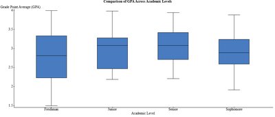
Example: The boxplot above compares GPA across academic levels (Freshman, Junior, Senior, Sophomore). It shows differences in median GPA, spread (IQR), and potential outliers between groups.

Z-Scores

Definition and Formula

A z-score tells how many standard deviations a data point is from the mean.

$z = \frac{x - \overline{x}}{s}$

• Positive z-score: value above the mean

• Negative z-score: value below the mean

• z = 0: value equals the mean

Applications of Z-Scores

• Identify outliers (z > 3 or z < -3)

• Standardize values for comparison across different scales

• Compute probabilities

Empirical Rule (68-95-99.7 Rule)

For bell-shaped (normal) distributions:

• 68% of data within 1 standard deviation of the mean

• 95% within 2 standard deviations

• 99.7% within 3 standard deviations

$\overline{x} \pm s$ $\overline{x} \pm 2s$ $\overline{x} \pm 3s$

Summary of Learning Outcomes

• Summarize categorical data using tables and charts

• Describe distribution shape, center, spread, and outliers

• Calculate and interpret mean, median, mode, range, IQR, and SD

• Choose appropriate measures based on distribution shape and outliers

• Identify outliers and interpret boxplots

• Use z-scores for comparison and outlier detection

• Apply the Empirical Rule to normal distributions