Describing and Summarizing Data in Introductory Statistics

Describing Data with Tables and Graphs

Ordered Arrays and Frequency Distributions

An ordered array is a sequence of data arranged from the smallest to the largest value. This arrangement helps to visualize the range of the data and can assist in identifying outliers. A frequency distribution is a summary table where data are grouped into intervals (classes), showing how many values fall into each interval. This condenses raw data into a more interpretable form and highlights where data are concentrated.

• Number of intervals: Should be between 5 and 15. Use the formula: $\text{Number of intervals} = 1 + 3.3 \log(n)$

• Interval width: $\text{Interval width} = \frac{\text{Range}}{\text{Number of intervals}}$

• Relative Frequency: $\text{Relative Frequency} = \frac{\text{Frequency}}{\text{Total}}$

• Percent: $\text{Percent} = \text{Relative Frequency} \times 100$

• Cumulative Frequency: Number of values in and below a particular category

• Cumulative Percentage: $\text{Cumulative Percentage} = \frac{\text{Cumulative Frequency}}{\text{Total}} \times 100$

Choosing class boundaries carefully is important, as different boundaries can change the appearance of the distribution, especially for small datasets.

Describing Data Numerically

Measures of Central Tendency

Measures of central tendency describe the center of a data set. The three main measures are the mean, median, and mode.

• Mean (Population): The arithmetic average of all values in the population.

The formula for the population mean is:

$\mu = \frac{\sum_{i=1}^{N} x_i}{N}$

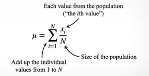
• Mean (Sample): The arithmetic average of all values in the sample.

$\bar{x} = \frac{\sum_{i=1}^{n} x_i}{n}$

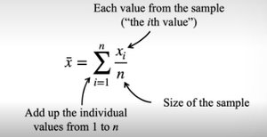
• Median: The middle value when data are ordered. For an odd number of observations, it is the middle value; for an even number, it is the average of the two middle values.

• Mode: The value that occurs most frequently in the data set. Useful for categorical, discrete, or binned continuous data.

Measures of Variability (Dispersion)

Measures of variability describe the spread of the data.

• Range: Difference between the maximum and minimum values.

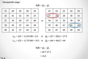
• Interquartile Range (IQR): Difference between the 75th percentile (Q3) and the 25th percentile (Q1).

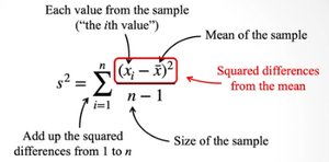
• Variance: Average of the squared differences from the mean.

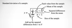
• Standard Deviation: Square root of the variance; describes the average distance of values from the mean.

Population variance formula:

$\sigma^2 = \frac{\sum_{i=1}^{N} (x_i - \mu)^2}{N}$

Sample variance formula:

$s^2 = \frac{\sum_{i=1}^{n} (x_i - \bar{x})^2}{n-1}$

Sample standard deviation formula:

$s = \sqrt{\frac{\sum_{i=1}^{n} (x_i - \bar{x})^2}{n-1}}$

Five Number Summary and Box Plots

The five number summary consists of the minimum, Q1, median (Q2), Q3, and maximum. A box plot graphically displays these values and highlights outliers.

Describing Data Graphically

Histograms and Distribution Shapes

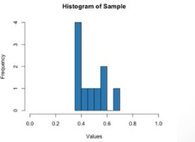
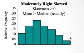
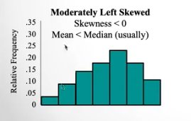
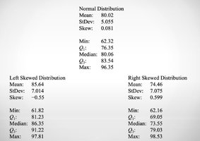
Histograms are used to visualize the distribution of data. The shape of the distribution can be symmetric, right-skewed, or left-skewed.

• Symmetric (Not Skewed): Mean = Median; Skewness = 0

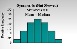
• Moderately Right Skewed: Mean > Median; Skewness > 0

• Moderately Left Skewed: Mean < Median; Skewness < 0

Measures of Distribution Shape

• Skewness: Measures the asymmetry of the distribution around the mean.

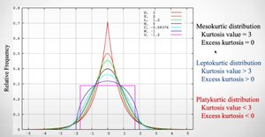
• Kurtosis: Measures the "tailedness" of the distribution (how likely it is to have extreme values).

Probability Distributions

Types of Variables

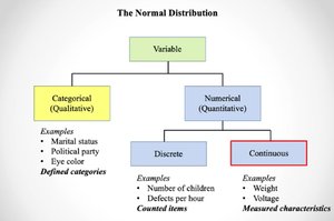
Variables can be classified as categorical (qualitative) or numerical (quantitative). Numerical variables can be discrete (counted) or continuous (measured).

Normal Distribution

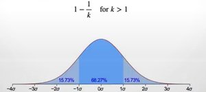
The normal distribution is a symmetric, bell-shaped curve defined by its mean ($\mu$) and standard deviation ($\sigma$). It is fundamental in inferential statistics.

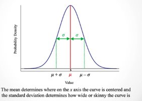
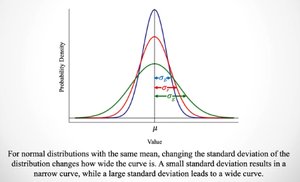
Changing the standard deviation alters the width of the curve, while the mean shifts its center.

The empirical rule states that for a normal distribution:

• 68% of data falls within 1 standard deviation of the mean

• 95% within 2 standard deviations

• 99.7% within 3 standard deviations

Sampling Distributions and the Central Limit Theorem

Sampling Distributions

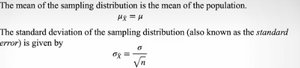
A sampling distribution is the probability distribution of a statistic (like the mean or proportion) based on all possible samples from a population. The mean of the sampling distribution of the sample mean is equal to the population mean, and its standard deviation (standard error) is $\sigma_{\bar{x}} = \frac{\sigma}{\sqrt{n}}$.

The Central Limit Theorem states that, for large enough sample sizes, the sampling distribution of the sample mean will be approximately normal, regardless of the population's distribution.

Calculating Z-scores for Sampling Distributions

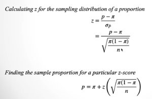
To standardize a sample mean or proportion, use the z-score formulas:

• For means: $z = \frac{\bar{x} - \mu}{\sigma_{\bar{x}}}$

• For proportions: $z = \frac{p - \pi}{\sigma_p}$

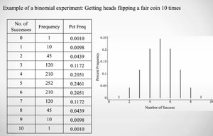
Binomial Distribution & Discrete Random Variables

Binomial Distribution

The binomial distribution models the number of successes in a fixed number of independent trials, each with the same probability of success ($\pi$). The mean and standard deviation of a binomial random variable $X$ are:

• $\mu = n\pi$

• $\sigma = \sqrt{n\pi(1-\pi)}$

Summary Table Example

The following table summarizes a probability distribution for the number of persons in a household:

Number of persons	Number of households (in millions)	Probability distribution	Cumulative probability
1	31.1	0.2681	0.2681
2	38.6	0.3328	0.6009
3	18.8	0.1621	0.7629
4	16.2	0.1397	0.9026
5	7.2	0.0621	0.9647
6	2.7	0.0233	0.9879
7 or more	1.4	0.0121	1.000

Evaluating Normality

To assess whether data are normally distributed, consider:

• Visual inspection (histogram, Q-Q plot)

• Descriptive statistics (mean ≈ median, skewness ≈ 0, kurtosis ≈ 3)

• Empirical rule (proportion of data within 1, 2, 3 standard deviations)

Additional info:

These notes cover the foundational concepts of describing and summarizing data, probability distributions, and the basics of inferential statistics, as required for an introductory statistics course.