Describing and Summarizing Data: Tables, Graphs, and Numerical Measures

Describing Data with Tables and Graphs

Frequency Distributions

A frequency distribution is a table that organizes data into classes or intervals, showing the number of observations in each class. This helps to summarize large data sets and identify patterns.

• Class Intervals: Ranges into which data are grouped (e.g., [5,10), [10,15), etc.).

• Class Width: The difference between the lower limits of consecutive classes.

• Frequency: The count of data points in each class.

Example: Student loan debt data grouped into 9 classes, such as [5,10), [10,15), etc., with frequencies showing how many students fall into each debt range.

Histograms

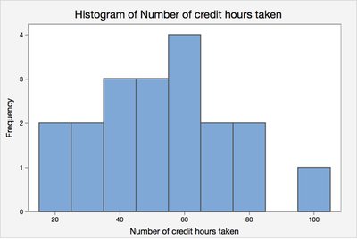
A histogram is a graphical representation of a frequency distribution for quantitative data. The x-axis shows the class intervals, and the y-axis shows the frequency.

• Frequency Histogram: Displays the number of observations in each class.

• Relative Frequency Histogram: Displays the proportion or percentage of observations in each class.

Example: The histogram below shows the distribution of the number of credit hours taken by students.

Bar Charts for Qualitative Data

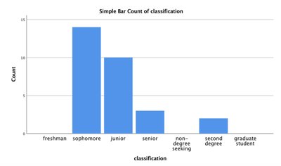
Bar charts are used to display the frequency of categories for qualitative (categorical) data. Each bar represents a category, and the height of the bar corresponds to the count or frequency.

Example: The bar chart below shows the classification of students (e.g., sophomore, junior, etc.) in a statistics class.

Describing Data Numerically

Measures of Central Tendency

Measures of central tendency describe the center or typical value of a data set.

• Mean (Arithmetic Average): $\bar{x} = \frac{\sum x_i}{n}$

• Median: The middle value when data are ordered from least to greatest.

• Mode: The value(s) that occur most frequently in the data set.

Example: For the weights of adults (e.g., 274, 235, 223, ...), calculate the mean, median, and mode. If an outlier (e.g., 290 lbs) is removed, recalculate the median to see the effect of outliers.

Weighted Mean

The weighted mean is used when different values in a data set contribute unequally to the final average. The formula is:

$\bar{x}_w = \frac{\sum w_i x_i}{\sum w_i}$

• Example: If homework counts for 15%, quizzes for 15%, and exams for 70% of a grade, and the averages are 94, 82, and 93, respectively, the weighted mean determines the final grade.

Shapes of Distributions

Common Distribution Shapes

Understanding the shape of a distribution helps in interpreting data and choosing appropriate statistical methods.

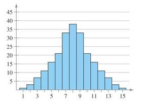
• Symmetric (Bell-shaped): Data are evenly distributed around the center.

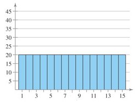
• Uniform: All values have approximately the same frequency.

• Skewed Right (Positively Skewed): Most data are on the left, with a long tail to the right.

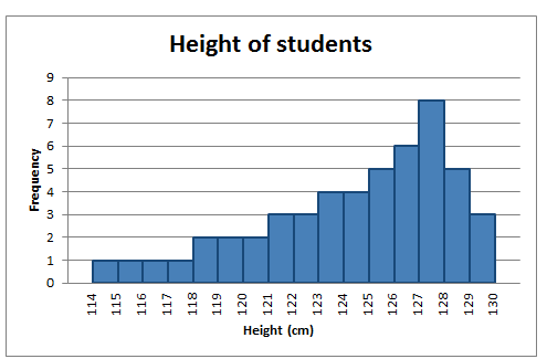
• Skewed Left (Negatively Skewed): Most data are on the right, with a long tail to the left.

Examples: The following images illustrate different distribution shapes:

Measures of Variation and Position

Measures of Variation (Spread)

Variation measures describe how spread out the data are.

• Range: $\text{Range} = \text{max} - \text{min}$

• Population Variance: $\sigma^2 = \frac{\sum (x - \mu)^2}{N}$

• Population Standard Deviation: $\sigma = \sqrt{\sigma^2}$

• Sample Variance: $s^2 = \frac{\sum (x - \bar{x})^2}{n-1}$

• Sample Standard Deviation: $s = \sqrt{s^2}$

Example: Compare the range and standard deviation of starting salaries at two corporations to determine which has more variability.

Empirical Rule

The Empirical Rule applies to bell-shaped (normal) distributions and estimates the proportion of data within 1, 2, or 3 standard deviations of the mean:

• About 68% within 1 standard deviation

• About 95% within 2 standard deviations

• About 99.7% within 3 standard deviations

Example: For women with mean height 64.2 inches and standard deviation 2.9 inches, estimate the percent of women above 70 inches or between 61.3 and 72.9 inches.

Chebyshev’s Theorem

Chebyshev’s Theorem states that for any data set (regardless of shape), the proportion of values within k standard deviations of the mean is at least $1 - \frac{1}{k^2}$ for $k > 1$.

• For $k=2$, at least 75% of data within 2 standard deviations

• For $k=3$, at least 88.9% of data within 3 standard deviations

Example: If the average age is 35.3 years with a standard deviation of 17.1 years, at least 75% of ages are between $35.3 - 2 \times 17.1$ and $35.3 + 2 \times 17.1$.

Percentiles and Quartiles

Percentiles indicate the relative standing of a value in a data set. The p-th percentile is the value below which p% of the data fall.

• Quartiles: Divide data into four equal parts:

  • Q1: 25th percentile

  • Q2: 50th percentile (median)

  • Q3: 75th percentile

Example: For the number of nuclear power plants in 15 countries, find Q1, Q2, and Q3 to describe the spread of the data.

Interquartile Range (IQR) and Outliers

The Interquartile Range (IQR) measures the spread of the middle 50% of data: $\text{IQR} = Q_3 - Q_1$.

• Outliers are values that fall below $Q_1 - 1.5 \times \text{IQR}$ or above $Q_3 + 1.5 \times \text{IQR}$.

Example: Use the IQR to determine if any countries are outliers in the number of nuclear power plants.

Five Number Summary and Boxplots

The five number summary consists of the minimum, Q1, median (Q2), Q3, and maximum. A box-and-whisker plot (boxplot) visually displays these values and highlights outliers.

Z-Scores

A z-score indicates how many standard deviations a value is from the mean.

• Sample z-score: $z = \frac{x - \bar{x}}{s}$

• Population z-score: $z = \frac{x - \mu}{\sigma}$

• z > 0: Value is above the mean; z < 0: Value is below the mean; z = 0: Value equals the mean.

Example: For SAT scores with mean 1263 and standard deviation 114, a score of 1377 has a z-score of $z = \frac{1377 - 1263}{114}$.

Scores with |z| > 2 are often considered unusual.

Summary Tables and Graphs

Descriptive Statistics Table Example

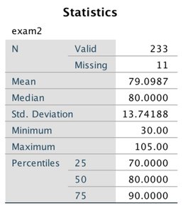
The following table summarizes key statistics for an exam:

Statistic	Value
Mean	79.10
Median	80.00
Standard Deviation	13.74
Minimum	30.00
Maximum	105.00
25th Percentile	70.00
50th Percentile	80.00
75th Percentile	90.00

Histogram Example

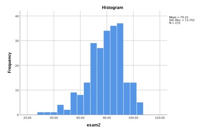
The histogram below shows the distribution of exam scores:

Another Descriptive Statistics Table Example

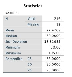
Statistic	Value
Mean	77.48
Median	80.00
Standard Deviation	18.82
Minimum	30.00
Maximum	105.00
25th Percentile	65.00
50th Percentile	80.00
75th Percentile	95.00

Histogram Example

The histogram below shows the distribution of another exam's scores:

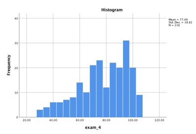
Additional info: These tables and histograms are used to summarize and visualize the distribution, central tendency, and spread of exam scores, which are key concepts in descriptive statistics.