Describing Data with Graphs: Categorical and Quantitative Variables

Chapter 2: Exploring Data with Graphs and Numerical Summaries

Section 2.2: How Can We Describe Data Using Graphical Summaries?

This section introduces the foundational graphical methods used in introductory statistics to summarize and interpret both categorical and quantitative data. Understanding these visual tools is essential for effective data analysis and communication.

Distribution

Understanding Distributions

A distribution describes the possible values a variable can take and how frequently each value occurs. Distributions can be represented visually using graphs or frequency tables, which help organize and summarize collected data.

• Frequency Table: Lists each value and the number of times it occurs.

• Relative Frequency: The proportion or percentage of observations for each value.

Example: If five friends can do 3, 1, 8, 3, and 5 push-ups, a frequency table would show how many times each number appears.

Graphs for Categorical Variables

Pie Charts

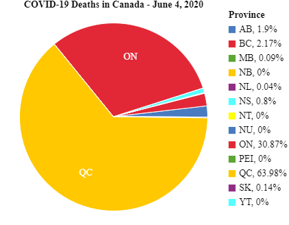
Pie charts are used to summarize categorical variables. Each category is represented as a slice of a circle, with the size of each slice proportional to the percentage of observations in that category.

• Best for showing the composition of a whole.

• Each slice's angle is calculated as: $\text{Angle} = \text{Percentage} \times 360^\circ$

Example: COVID-19 deaths in Canada by province, June 4, 2020.

Bar Graphs

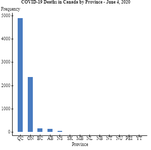
Bar graphs display a vertical bar for each category, with the height representing either the count (frequency) or percentage (relative frequency) for that category. Bar graphs are often easier than pie charts for comparing categories.

• Bars are separated to emphasize categorical nature.

• Can be used for both counts and percentages.

Example: COVID-19 deaths in Canada by province, June 4, 2020 (bar graph).

Pareto Charts

A Pareto chart is a bar graph where categories are ordered by frequency, from highest to lowest. This helps highlight the most significant categories.

Class Exercise Example

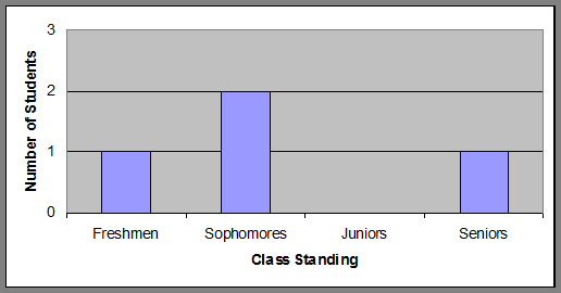
Given a bar graph of class standings (Freshmen, Sophomores, Juniors, Seniors), you can determine the number of students in each category by reading the bar heights.

Real-World Example: Leading Causes of Death in Canada

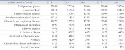
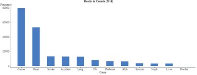
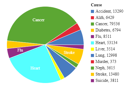
Tabular and graphical summaries can be used to compare causes of death over time or by category.

Leading causes of death	2014	2015	2016	2017	2018
Malignant neoplasms	77059	77054	79046	79384	79536
Diseases of heart	51014	51534	51396	53039	53134
Cerebrovascular diseases	13573	13785	13553	13389	13480
Accidents (unintentional injuries)	11724	11833	11931	13594	13290
Chronic lower respiratory diseases	11876	12173	12293	13238	12998
Influenza and pneumonia	6977	7630	6295	7389	8511
Diabetes mellitus	7071	7171	6888	6887	6794
Alzheimer's disease	6410	6587	6823	6675	6429
Intentional self-harm (suicide)	4025	4126	4154	4005	3811
Nephritis	3098	3129	3385	3475	3615
Chronic liver disease and cirrhosis	3126	3176	3385	3475	3514
Assault (homicide)	439	456	386	459	373

Graphs for Quantitative Data

Dot Plots

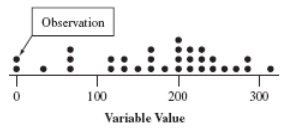
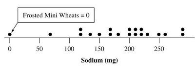
Dot plots are used for small data sets of quantitative variables. Each observation is represented by a dot placed above its value on a number line. Dot plots retain all individual data values and are useful for detecting clusters and gaps.

• Draw a horizontal line and label it with the variable name.

• Mark regular values and place a dot for each observation.

Example: Dot plot for sodium content in cereals.

Stem-and-Leaf Plots

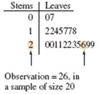
Stem-and-leaf plots are another way to summarize quantitative data, especially for small to moderate data sets. Each value is split into a "stem" (all but the last digit) and a "leaf" (the last digit). Stems are listed in a column, and leaves are written in rows beside their stems.

• Retain all original data values.

• Show the shape and distribution of the data.

Histograms

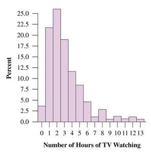
A histogram is a bar graph for quantitative data, showing the frequency or relative frequency of observations within specified intervals (bins). Histograms are best for large data sets and provide a compact summary of the data's distribution.

• Divide the range into equal-width intervals.

• Count the number of observations in each interval.

• Draw bars with heights corresponding to frequencies or percentages.

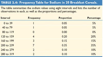
Example: Frequency table for sodium in 20 breakfast cereals.

Interval	Frequency	Proportion	Percentage
0 to 39	1	0.05	5%
40 to 79	1	0.05	5%
80 to 119	0	0.00	0%
120 to 159	4	0.20	20%
160 to 199	3	0.15	15%
200 to 239	7	0.35	35%
240 to 279	2	0.10	10%
280 to 319	2	0.10	10%

Interpreting Histograms

Key Features: Center, Spread, and Shape

When interpreting histograms, focus on three main features:

• Center: Where the distribution is centered (e.g., median or mean).

• Spread: The variability or range of the data.

• Shape: The overall appearance—symmetric, skewed left, or skewed right.

Skewness:

• Skewed to the left: Left tail is longer (few low values).

• Skewed to the right: Right tail is longer (few high values).

• Symmetric: Both sides are mirror images.

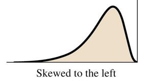
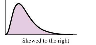
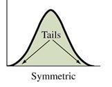
Examples of Skewness:

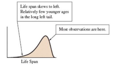
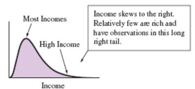
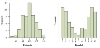
Types of Mounds: Distributions can be unimodal (one peak) or bimodal (two peaks).

Outliers

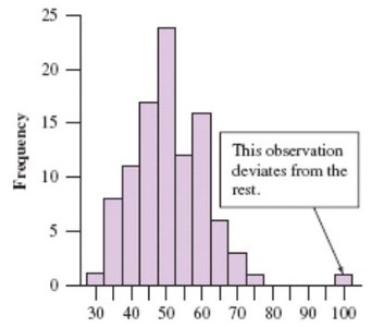
An outlier is an observation that falls far from the rest of the data. Outliers should be investigated as they may indicate variability, errors, or interesting phenomena.

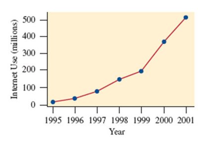
Time Plots

Displaying Data Over Time

Time plots are used for data collected over time (time series). Each observation is plotted against the time it was measured, and points are usually connected to show trends or patterns.

• Horizontal axis: Time

• Vertical axis: Variable of interest

• Look for trends, cycles, or unusual patterns

Lesson Summary

• Descriptive statistics use graphical and numerical methods to summarize data.

• Categorical variables are summarized with pie charts and bar graphs.

• Quantitative variables are summarized with dot plots, stem-and-leaf plots, histograms, and box plots.

• Key features to identify: shape (symmetrical or skewed), center, spread, and outliers.