Describing Data with Tables and Graphs: Frequency Distributions, Graphical Displays, and Measures of Central Tendency

Describing Data with Tables and Graphs

Frequency Distributions

A frequency distribution is a table that organizes data into classes or intervals, showing the number of data entries (frequency) in each class. This method helps summarize large data sets and reveals patterns in the data.

• Class limits: The smallest and largest data values that can belong to a class.

• Class width: The difference between the lower limits of consecutive classes. Calculated as: $\text{Class width} = \frac{X_{\text{max}} - X_{\text{min}}}{\text{Number of classes}}$ (always round up to the next whole number).

• Steps to construct a frequency distribution:

  1. Decide on the number of classes (usually 5 to 20).

  2. Find the class width.

  3. Determine the class limits.

  4. Tally the data into classes.

  5. Count the tallies to find the frequency for each class.

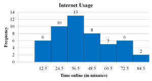
Example: Internet usage times for 50 subscribers are grouped into 7 classes. The class width is calculated as $\frac{86-7}{7} \approx 11.3$, rounded up to 12.

Frequency Histogram

A frequency histogram is a bar graph representing the frequency distribution. The horizontal axis shows the data values (quantitative), and the vertical axis shows the frequencies. Bars are adjacent to indicate continuous data.

Relative Frequency Histogram

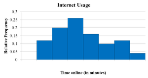
A relative frequency histogram displays the same data as a frequency histogram, but the vertical axis shows the proportion (or percentage) of data in each class rather than the count. This allows for comparison between data sets of different sizes.

Stem-and-Leaf Plot

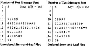
A stem-and-leaf plot is a method of displaying quantitative data where each value is split into a "stem" (all but the final digit) and a "leaf" (the final digit). This plot retains the original data values and shows the distribution's shape.

• Unordered and ordered versions can be constructed for clarity.

Dot Plot

A dot plot displays each data value as a dot above a number line. It is useful for small to moderate-sized data sets and shows clusters, gaps, and outliers.

Pie Chart

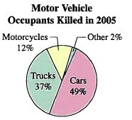
A pie chart is a circular graph divided into sectors, each representing a category's relative frequency. The area of each sector is proportional to the frequency or percentage of the category.

Pareto Chart

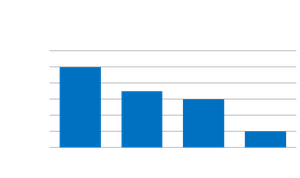
A Pareto chart is a vertical bar graph where bars represent frequencies or relative frequencies of categories, arranged in decreasing order. It is useful for identifying the most significant factors in a data set.

Scatter Plot

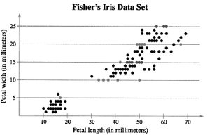
A scatter plot graphs paired data as points in a coordinate plane, showing the relationship between two quantitative variables. Patterns may indicate correlation (positive, negative, or none).

Time Series Chart

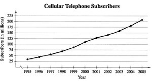
A time series chart displays data points collected or recorded at specific time intervals. It is useful for identifying trends over time.

Measures of Central Tendency

Mean

The mean (average) is the sum of all data entries divided by the number of entries. It is sensitive to outliers.

• Population mean: $\mu = \frac{\sum x}{N}$

• Sample mean: $\bar{x} = \frac{\sum x}{n}$

Median

The median is the middle value when the data set is ordered. If the number of entries is even, the median is the mean of the two middle values. The median is less affected by outliers than the mean.

Mode

The mode is the data value that occurs most frequently. A data set may have no mode, one mode (unimodal), or more than one mode (bimodal or multimodal).

Comparing Mean, Median, and Mode

The mean uses all data values but is affected by outliers. The median is robust to outliers. The mode may not represent the center if the data is skewed or multimodal.

Shape of Distributions

Symmetric Distribution

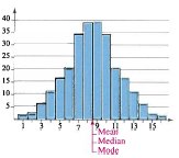
A symmetric distribution has mirror-image halves when split down the center. The mean, median, and mode are all approximately equal.

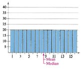
Uniform Distribution

A uniform distribution (rectangular) has all classes with equal or nearly equal frequencies. The mean and median are at the center.

Skewed Distributions

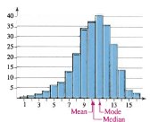
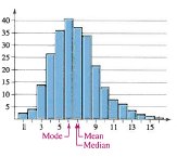
• Skewed Left (Negative Skew): The "tail" extends to the left. Mean < Median < Mode.

• Skewed Right (Positive Skew): The "tail" extends to the right. Mean > Median > Mode.

Measures of Variation

Range

The range is the difference between the maximum and minimum values in a data set: $\text{Range} = X_{\text{max}} - X_{\text{min}}$. It is easy to compute but only uses two data values.

Variance and Standard Deviation

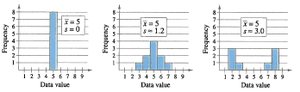
Variance measures the average squared deviation from the mean. Standard deviation is the square root of the variance and measures the typical distance of data values from the mean.

• Population variance: $\sigma^2 = \frac{\sum (x - \mu)^2}{N}$

• Population standard deviation: $\sigma = \sqrt{\frac{\sum (x - \mu)^2}{N}}$

• Sample variance: $s^2 = \frac{\sum (x - \bar{x})^2}{n-1}$

• Sample standard deviation: $s = \sqrt{\frac{\sum (x - \bar{x})^2}{n-1}}$

Empirical Rule (68-95-99.7 Rule)

For bell-shaped (normal) distributions:

• About 68% of data lie within 1 standard deviation of the mean.

• About 95% within 2 standard deviations.

• About 99.7% within 3 standard deviations.

Chebychev’s Theorem

For any data set (regardless of shape), at least $1 - \frac{1}{k^2}$ of the data lie within $k$ standard deviations of the mean ($k > 1$). For $k=2$, at least 75% of data; for $k=3$, at least 89% of data.

Measures of Position

Quartiles and Interquartile Range (IQR)

Quartiles divide ordered data into four equal parts:

• Q1: 25th percentile

• Q2: 50th percentile (median)

• Q3: 75th percentile

The interquartile range (IQR) is $Q_3 - Q_1$ and measures the spread of the middle 50% of data.

Box-and-Whisker Plot

A box-and-whisker plot visually displays the five-number summary: minimum, Q1, median (Q2), Q3, and maximum. It highlights the central tendency, spread, and potential outliers.

Standard Score (Z-Score)

The z-score indicates how many standard deviations a value $x$ is from the mean $\mu$:

$z = \frac{x - \mu}{\sigma}$

• Negative z: value is below the mean

• Positive z: value is above the mean

• z = 0: value equals the mean

Unusual scores (|z| > 2) occur about 5% of the time; very unusual scores (|z| > 3) about 0.3% of the time.