Describing Data with Tables and Graphs: Frequency Distributions and Graphical Representations

Describing Data with Tables and Graphs

Frequency Distributions

A frequency distribution is a table that lists each category of data and the number of occurrences for each category. This is a fundamental method for organizing data, especially qualitative (categorical) data, to reveal patterns and facilitate further analysis.

• Frequency: The count of occurrences for each category.

• Relative Frequency: The proportion of occurrences for each category, calculated as frequency divided by the sample size.

• Relative Frequency Distribution: A listing of all values that a variable can take, together with their relative frequencies.

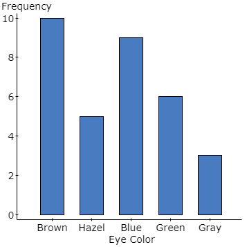
• Example: Eye color data for a sample of 33 individuals, categorized and tallied.

Eye Color	Frequency	Relative Frequency
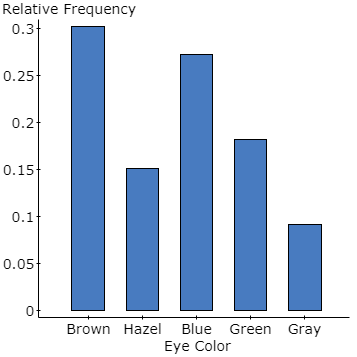
Brown	10	10/33 ≈ 0.3030
Hazel	5	5/33 ≈ 0.1515
Blue	9	9/33 ≈ 0.2727
Green	6	6/33 ≈ 0.1818
Gray	3	3/33 ≈ 0.0909

Bar Graphs

A bar graph visually represents categorical data by labeling each category on one axis and the frequency or relative frequency on the other axis. Bars are separated to emphasize the discrete nature of the categories.

Relative Frequency Bar Graphs

Relative frequency bar graphs display the proportion of each category, making it easier to compare categories when sample sizes differ.

Pareto Charts

A Pareto chart is a bar graph where bars are arranged in decreasing order of frequency or relative frequency. This helps highlight the most common categories.

Pie Charts

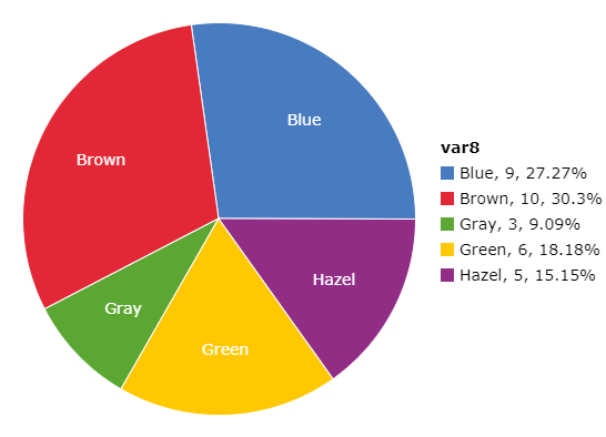
A pie chart divides a circle into sectors, each representing a category. The area of each sector is proportional to the frequency or relative frequency of the category.

Graphs for Quantitative Data

Quantitative data can be visualized using several types of graphs, each suited to different data characteristics and analysis goals.

Histograms

A histogram is constructed by drawing rectangles for each class of data. The height of each rectangle represents the frequency or relative frequency, and the rectangles touch each other to indicate the continuous nature of the data.

• Frequency Histogram: Shows the count of data points in each class.

• Relative Frequency Histogram: Shows the proportion of data points in each class.

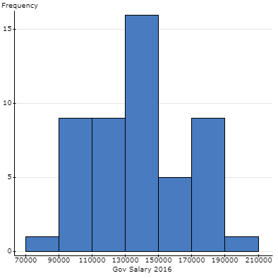
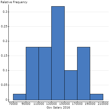
Classes and Class Limits

• Class: A category into which data are grouped.

• Lower Class Limit: The smallest value in a class.

• Upper Class Limit: The largest value in a class.

• Class Midpoint: Calculated as $(\text{Lower Limit} + \text{Upper Limit}) / 2$.

• Class Width: The difference between two consecutive lower class limits.

Cumulative Frequency and Cumulative Relative Frequency Distributions

A cumulative frequency distribution displays the aggregate frequency up to each class. A cumulative relative frequency distribution shows the proportion of observations up to each class.

Class	Frequency	Class Midpoint	Relative Frequency	Cumulative Frequency	Cumulative Relative Frequency
$70,000-89,999$	1	$80,000$	0.02	1	0.02
$90,000-109,999$	9	$100,000$	0.18	10	0.20
$110,000-129,999$	9	$120,000$	0.18	19	0.38
$130,000-149,999$	15	$140,000$	0.30	34	0.68
$150,000-169,999$	5	$160,000$	0.10	39	0.78
$170,000-189,999$	10	$180,000$	0.20	49	0.98
$190,000-209,999$	1	$200,000$	0.02	50	1.00

Frequency Polygons

A frequency polygon uses points connected by line segments to represent frequencies for classes. Points are plotted above each class midpoint, and the graph is closed by connecting the ends to the horizontal axis.

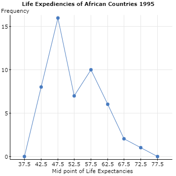
Ogives

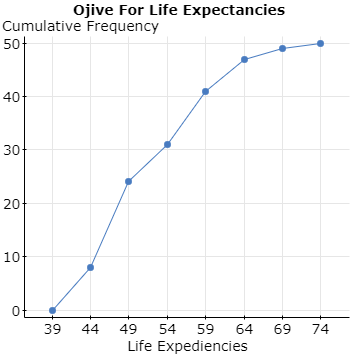
An ogive is a graph that represents cumulative frequency or cumulative relative frequency for the classes. Points are plotted at the upper class limits, and line segments connect these points.

Stem-and-Leaf Diagrams

Stem-and-leaf diagrams are useful for data sets with many repeated values or values within a similar range. The stem is the first digit(s), and the leaf is the last digit of each number.

• Example: Life expectancy data for African countries, 1995.

Dot Plots

Dot plots display each data point as a dot, often used for small data sets or those with many repeated values. Data is not grouped, and each dot represents a single observation.

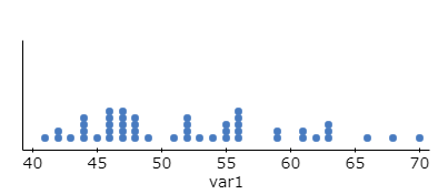
Time Series Plots

A time series plot is used to visualize how a variable changes over time. The horizontal axis represents time, and the vertical axis represents the variable of interest. Points are connected by line segments.

Best Practices for Graphs

• Clearly define how data is grouped.

• Use clear and even scales.

• Include units in the graph.

• Ensure graphs are easy to read and accurately represent the data set.

Summary Table: Types of Graphs and Their Uses

Graph Type	Data Type	Main Purpose
Bar Graph	Qualitative	Compare frequencies or proportions across categories
Pareto Chart	Qualitative	Highlight most frequent categories
Pie Chart	Qualitative	Show proportion of each category
Histogram	Quantitative	Show distribution of data
Frequency Polygon	Quantitative	Show shape of distribution
Ogive	Quantitative	Show cumulative frequencies
Stem-and-Leaf	Quantitative	Display individual values and distribution
Dot Plot	Quantitative	Show individual data points
Time Series Plot	Quantitative (over time)	Show trends over time

Additional info: The notes cover the essentials of Chapter 2: Describing Data with Tables and Graphs, including both qualitative and quantitative graphical methods, and best practices for accurate data representation.