Describing the Relation Between Two Variables: Scatter Diagrams, Correlation, and Least-Squares Regression

Chapter 4: Describing the Relation Between Two Variables

Section 4.1: Scatter Diagrams and Correlation

In statistics, understanding the relationship between two quantitative variables is essential for data analysis. This section introduces graphical and numerical methods for describing such relationships, focusing on scatter diagrams and the correlation coefficient.

Univariate vs. Bivariate Data

• Univariate data: Data in which a single variable is measured for each individual.

• Bivariate data: Data in which two variables are measured on each individual, allowing us to study the relationship between them.

We are often interested in how changes in one variable (the explanatory variable or independent variable) affect another variable (the response variable or dependent variable).

• Explanatory variable: The variable we control or believe explains changes in the response variable.

• Response variable: The variable that changes as a result of changes in the explanatory variable.

Example: A marketing firm studies the relationship between hours of television advertising (explanatory variable) and product sales (response variable).

Scatter Diagrams

A scatter diagram is a graphical tool used to display the relationship between two quantitative variables. Each point represents an individual’s values for both variables.

• The response (dependent) variable is plotted on the y-axis.

• The explanatory (independent) variable is plotted on the x-axis.

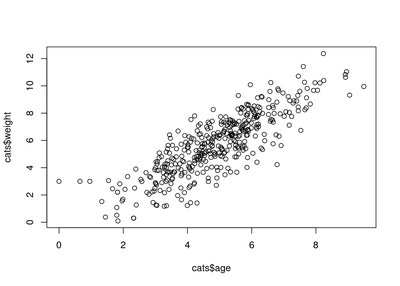
Scatter diagrams help us visually identify trends, such as linear or nonlinear patterns, and the direction (positive or negative) of the relationship.

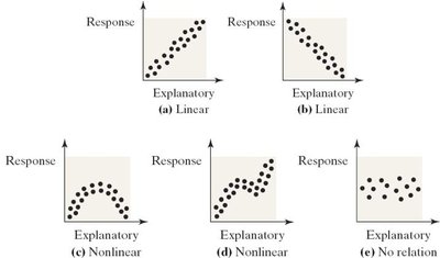
Interpreting Scatter Diagrams

• Linear pattern: Points fall roughly along a straight line.

• Curved (nonlinear) pattern: Points follow a curved path.

• No pattern: Points are scattered randomly, indicating no relationship.

• Positive relationship: As x increases, y increases (upward slope).

• Negative relationship: As x increases, y decreases (downward slope).

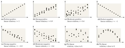
Correlation Coefficient (r)

The linear correlation coefficient (Pearson’s r) is a numerical measure of the strength and direction of the linear relationship between two quantitative variables.

• Population correlation coefficient: $\rho$ (rho)

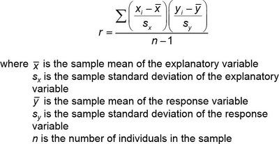
• Sample correlation coefficient: $r$

The formula for the sample correlation coefficient is:

$r = \frac{\sum \left( \frac{x_i - \overline{x}}{s_x} \right) \left( \frac{y_i - \overline{y}}{s_y} \right)}{n-1}$

Properties of the Correlation Coefficient

• r is always between -1 and 1, inclusive.

• r = 1: Perfect positive linear relationship.

• r = -1: Perfect negative linear relationship.

• r close to 0: Little or no linear relationship.

• The closer r is to ±1, the stronger the linear relationship.

• r is unitless and unaffected by the units of measurement.

• r is sensitive to outliers, which can distort the value.

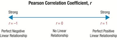
Examples of Correlation Strength and Direction

Calculating the Correlation Coefficient

Correlation can be calculated using statistical software or calculators. For example, using a TI-83/84 calculator or StatCrunch, you can input the data and use built-in functions to compute r.

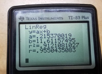
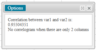
Testing for a Linear Relation

To determine if a linear relationship exists, compare the absolute value of r to a critical value from a table based on sample size (n). If |r| is greater than the critical value, a significant linear relationship exists.

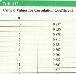
Correlation vs. Causation

Correlation does not imply causation. A high correlation between two variables does not mean that changes in one cause changes in the other. Correlation can be due to:

• Coincidence

• Lurking variables (third variables affecting both)

• Trends in time series data

Example: A high correlation between cheese consumption and deaths by bedsheet entanglement does not imply causation.

Section 4.2: Least-Squares Regression

Once a linear relationship is established, we can model it with a linear equation using the method of least squares regression. This allows us to predict values and understand the relationship quantitatively.

Finding the Least-Squares Regression Line

The least-squares regression line is the line that minimizes the sum of the squared differences (residuals) between observed and predicted values of the response variable.

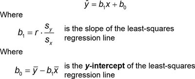
The equation of the least-squares regression line is:

$\hat{y} = b_1 x + b_0$

• $b_1$ is the slope: $b_1 = r \cdot \frac{s_y}{s_x}$

• $b_0$ is the y-intercept: $b_0 = \overline{y} - b_1 \overline{x}$

Calculating and Interpreting the Regression Line

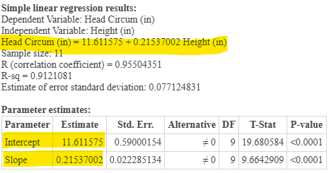
Given summary statistics and the correlation coefficient, you can compute the regression line. For example, with head circumference (y) and height (x) data:

• Mean of x ($\overline{x}$): 26.455

• Standard deviation of x ($s_x$): 1.0944

• Mean of y ($\overline{y}$): 17.309

• Standard deviation of y ($s_y$): 0.235

• Correlation coefficient (r): 0.955

The regression equation is:

$\text{Head Circumference (in)} = 11.611575 + 0.21537002 \times \text{Height (in)}$

Interpreting Slope and Intercept

• Slope: For each one-unit increase in the explanatory variable, the response variable increases by the value of the slope.

• Intercept: The predicted value of the response variable when the explanatory variable is zero. Interpretation depends on whether zero is a meaningful value for the explanatory variable.

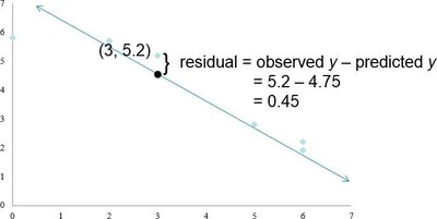
Residuals

A residual is the difference between the observed value and the predicted value from the regression line:

$\text{residual} = \text{observed } y - \text{predicted } y$

Using the Regression Line for Prediction

The regression line can be used to predict the response variable for values of the explanatory variable within the range of observed data. Predictions outside this range (extrapolation) are unreliable.

Summary Table: Steps for Least-Squares Regression

Step	Description
1	Calculate means and standard deviations for both variables
2	Compute the correlation coefficient (r)
3	Calculate the slope ($b_1$) and intercept ($b_0$)
4	Write the regression equation
5	Interpret the slope and intercept
6	Use the equation for prediction (within the scope of the data)

Cautions in Regression Analysis

• Do not use the regression line to predict values outside the observed range (extrapolation).

• Check for outliers, as they can significantly affect the regression line.

• Remember that correlation does not imply causation.

Key Terms and Concepts

• Bivariate data

• Explanatory variable

• Response variable

• Scatter diagram

• Correlation coefficient (r)

• Least-squares regression line

• Residual

• Lurking variable

• Extrapolation