Describing the Relation Between Two Variables: Scatter Diagrams and Correlation

Study Guide - Smart Notes

Tailored notes based on your materials, expanded with key definitions, examples, and context.

Chapter 4: Describing the Relation Between Two Variables

Univariate and Bivariate Data

In statistics, data can be classified based on the number of variables measured for each individual. Univariate data involves a single variable measured per individual, while bivariate data involves two variables measured on the same individual. Bivariate data allows us to explore relationships between variables.

Univariate Example: Measuring daily temperature at noon for each day in September.
Bivariate Example: Recording both hours of study and GPA for each student.

Scatter Diagrams (Scatter Plots)

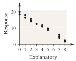
A scatter diagram (or scatter plot) is a graphical tool used to display the relationship between two quantitative variables measured on the same individuals. Each point on the plot represents one individual, with the explanatory variable on the x-axis and the response variable on the y-axis.

Explanatory Variable (x): The variable that explains or influences changes in the response variable.
Response Variable (y): The variable whose value is influenced by the explanatory variable.

Example scatter plot with labeled axes

Correlation

Correlation measures the strength and direction of the linear relationship between two quantitative variables. The data are represented as ordered pairs (x, y). The correlation coefficient is a unitless statistic that summarizes this relationship.

Sample correlation coefficient: Denoted by r.
Population correlation coefficient: Denoted by \( \rho \) (rho).
Properties: Correlation is not resistant to outliers and is only appropriate for linear relationships.

Interpreting the Correlation Coefficient

The correlation coefficient (r) ranges from -1 to 1:

r = 1: Perfect positive linear correlation
r = -1: Perfect negative linear correlation
r ≈ 0: No linear correlation

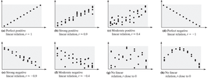
Examples of scatter plots with different correlation coefficients

Examples of Correlation Coefficient Values

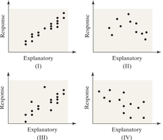
Strong positive correlation: r close to 1
Strong negative correlation: r close to -1
Weak or no correlation: r close to 0

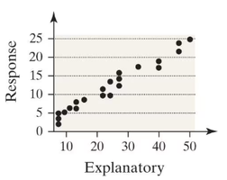
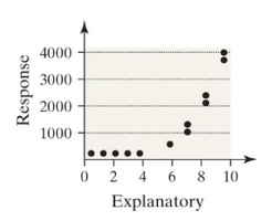
Scatter plots with various correlation coefficients Scatter plot with strong positive correlation Scatter plot with strong negative correlation Scatter plots with moderate and no correlation

Testing for Linear Relation Between Two Variables

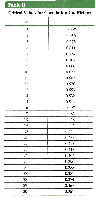
To determine if a linear relationship exists in the population, we use the sample correlation coefficient (r) and compare it to a critical value from a table based on the sample size (n) and the desired significance level.

Determine the sample size, n.
Find the critical value for r from the correlation coefficient table.
If |r| is greater than the critical value, conclude that a significant linear relationship exists.

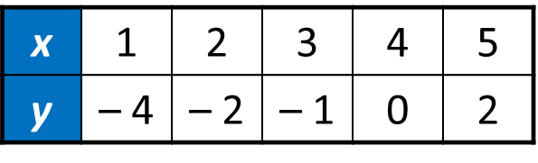
Critical values table for correlation coefficient

Example Table: Sample Data

x	1	2	3	4	5
y	-4	-2	-1	0	2

Using Technology: Statcrunch Example

Statistical software such as Statcrunch can be used to compute the correlation coefficient efficiently. The steps typically involve selecting the variables, choosing the correlation function, and interpreting the output.

Statcrunch correlation computation example

Correlation vs. Causation

It is important to note that correlation does not imply causation. Even if two variables are strongly correlated, this does not mean that changes in one variable cause changes in the other. There may be lurking variables or confounding factors that influence both variables.

Example: Ice cream sales and crime rates both increase in summer, but temperature is a lurking variable.
Example: Higher education levels and births to unmarried mothers are correlated due to both increasing over time, not because one causes the other.

Practice and Application Examples

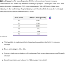
Example: Credit Scores and Interest Rates

Credit scores and interest rates example

Identify explanatory and response variables.
Draw a scatter diagram.
Calculate the correlation coefficient.
Interpret the existence of a linear relationship.

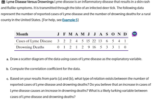
Example: Lyme Disease and Drowning Deaths

Lyme disease and drowning deaths example

Draw a scatter diagram using cases of Lyme disease as the explanatory variable.
Compute the correlation coefficient.
Discuss the presence of a lurking variable and the lack of causation.

Example: Crime Rate and Cell Phones

The linear correlation between violent crime rate and the percentage of the population with a cell phone is -0.013 for years since 1995. This weak correlation does not imply that increasing cell phone usage will decrease violent crime rates. A lurking variable may be influencing both variables.

Additional info: In all cases, it is essential to consider the context, possible lurking variables, and whether the relationship is truly linear before drawing conclusions from correlation analysis.