Descriptive Statistics: Data Classification, Central Tendency, Dispersion, and Position

Data and Statistics

Definition and Types of Data

Statistics is the science of collecting, organizing, analyzing, and interpreting data to make decisions. Data can be classified as either qualitative (categorical) or quantitative (numerical).

• Qualitative Data: Consists of attributes, labels, or non-numerical entries. Examples include gender, ethnicity, or group membership.

• Quantitative Data: Consists of numerical measurements or counts. Examples include height, weight, or GPA.

• Discrete Variable: Quantitative, countable numbers (e.g., number of children).

• Continuous Variable: Quantitative, measurable, can take decimals (e.g., height).

Branches of Statistics

Statistics is divided into two main branches:

• Descriptive Statistics: Involves the organization, summarization, and display of data.

• Inferential Statistics: Uses a sample to draw conclusions about a population.

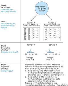
Example: Comparing two teaching methods using test scores from samples of first-grade children. Descriptive statistics summarize the average scores, while inferential statistics interpret whether the difference is meaningful for the population.

Describing Data Numerically

Measures of Central Tendency

Measures of central tendency describe the location of the data's center. The three most common are mean, median, and mode.

• Mean: The arithmetic average. For a population, $\mu = \frac{\sum x}{N}$; for a sample, $\bar{x} = \frac{\sum x}{n}$.

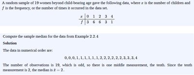
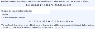
• Median: The middle value when data are ordered. If n is odd, the median is the middle value; if n is even, it is the average of the two middle values.

• Mode: The value that occurs most frequently. If no value repeats, there is no mode.

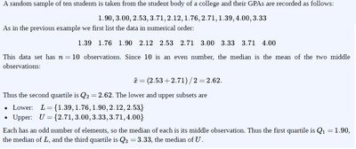
Example: For a sample of 19 women, the median is the tenth value in the ordered list. For a sample of 10 GPAs, the median is the average of the fifth and sixth values.

Note: The mean is sensitive to outliers, while the median is not.

Shapes of Distributions

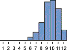
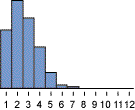
The shape of a distribution affects the relationship between mean, median, and mode.

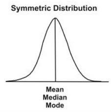
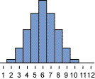
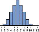
• Symmetric Distribution: Mean = Median = Mode.

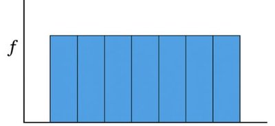
• Uniform Distribution: All values have equal frequency.

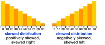
• Skewed Distribution: If the tail is longer on one side, the distribution is skewed left (mean < median) or skewed right (mean > median).

Measures of Dispersion

Range

The range is the difference between the maximum and minimum values in a data set.

• Formula: Range = Maximum - Minimum

• Disadvantage: Sensitive to outliers and ignores data distribution.

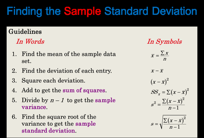
Variance and Standard Deviation

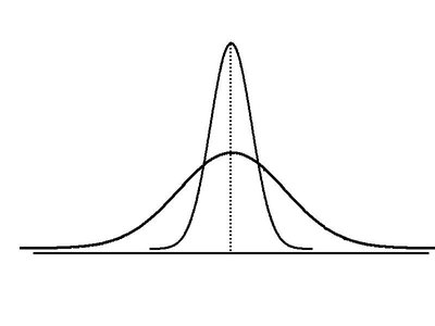
Variance and standard deviation measure the spread of data around the mean.

• Population Variance: $\sigma^2 = \frac{\sum (x - \mu)^2}{N}$

• Population Standard Deviation: $\sigma = \sqrt{\frac{\sum (x - \mu)^2}{N}}$

• Sample Variance: $s^2 = \frac{\sum (x - \bar{x})^2}{n-1}$

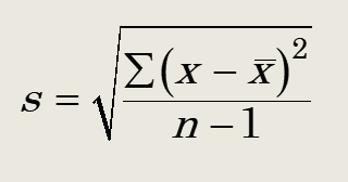
• Sample Standard Deviation: $s = \sqrt{\frac{\sum (x - \bar{x})^2}{n-1}}$

Interpretation: A larger standard deviation indicates greater spread in the data. Comparing standard deviations helps assess variability between data sets.

Coefficient of Variation (CV)

The coefficient of variation expresses the standard deviation as a percentage of the mean, allowing comparison between data sets with different units.

• Population CV: $CV = \frac{\sigma}{\mu} \times 100\%$

• Sample CV: $CV = \frac{s}{\bar{x}} \times 100\%$

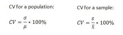
Example: Two stocks with the same standard deviation but different means have different CVs, indicating relative variability.

Measures of Position

Quartiles and Interquartile Range (IQR)

Quartiles divide ordered data into four equal parts. The interquartile range measures the spread of the middle 50% of the data.

• Q1: Median of the lower half

• Q2: Median

• Q3: Median of the upper half

• Interquartile Range: $IQR = Q3 - Q1$

Example: For a sample of 10 GPAs, Q1 = 1.90, Q2 = 2.62, Q3 = 3.33.

Box-and-Whisker Plot

A box-and-whisker plot visually displays the five-number summary: minimum, Q1, median (Q2), Q3, and maximum. It highlights the spread and potential outliers in the data.

Outliers

Outliers are data points that fall outside the expected range. They can be identified using the following rule:

• Lower Bound: $Q1 - 1.5 \times (Q3 - Q1)$

• Upper Bound: $Q3 + 1.5 \times (Q3 - Q1)$

Values outside these bounds are considered possible outliers.

Summary Table: Measures of Location and Dispersion

Measure	Definition	Formula
Mean	Arithmetic average	$\bar{x} = \frac{\sum x}{n}$
Median	Middle value	Position: $\frac{n+1}{2}$
Mode	Most frequent value	—
Range	Difference between max and min	Range = Max - Min
Variance	Average squared deviation	$s^2 = \frac{\sum (x - \bar{x})^2}{n-1}$
Standard Deviation	Square root of variance	$s = \sqrt{\frac{\sum (x - \bar{x})^2}{n-1}}$
Coefficient of Variation	Relative variation (%)	$CV = \frac{s}{\bar{x}} \times 100\%$
Interquartile Range	Spread of middle 50%	$IQR = Q3 - Q1$