Descriptive Statistics: Frequency Distributions, Graphs, and Measures of Central Tendency

Descriptive Statistics

Frequency Distributions and Their Graphs

Frequency distributions are fundamental tools in statistics for organizing and summarizing data. They display how data values are distributed across different intervals or classes, making it easier to identify patterns and trends.

• Frequency Distribution: A table showing classes or intervals of data with the count (frequency) of entries in each class.

• Class Limits: The smallest and largest values that can belong to each class.

• Class Width: The difference between the upper and lower class limits. Calculated as $\text{Class Width} = \frac{\text{Range}}{\text{Number of Classes}}$ (rounded up).

• Midpoint: The average of the lower and upper class limits: $\text{Midpoint} = \frac{\text{Lower Class Limit} + \text{Upper Class Limit}}{2}$

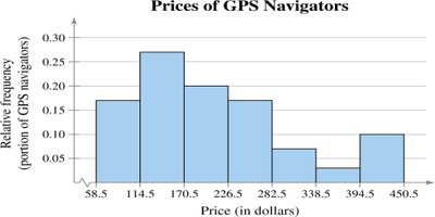
• Relative Frequency: The proportion of data in each class: $\text{Relative Frequency} = \frac{\text{Class Frequency}}{\text{Sample Size}}$

• Cumulative Frequency: The sum of the frequency for a class and all previous classes.

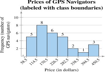
• Class Boundaries: Values that separate classes without gaps, calculated by averaging the upper limit of one class and the lower limit of the next.

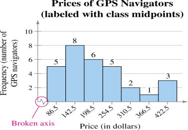
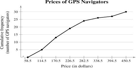
Example: Constructing a frequency distribution for GPS navigator prices involves determining class width, class limits, tallying data, and calculating frequencies, midpoints, relative frequencies, and cumulative frequencies.

Frequency Histogram

A frequency histogram is a bar graph representing the frequency distribution. The horizontal axis shows data values, and the vertical axis shows frequencies. Bars touch each other, indicating continuous data.

Frequency Polygon

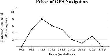
A frequency polygon is a line graph that connects the midpoints of each class, emphasizing the continuous change in frequencies. The graph starts and ends at the horizontal axis, extending one class width beyond the first and last midpoints.

Relative Frequency Histogram

This graph is similar to a frequency histogram but uses relative frequencies on the vertical axis. It helps compare distributions with different sample sizes.

Cumulative Frequency Graph (Ogive)

An ogive is a line graph displaying cumulative frequencies at each upper class boundary. It shows how many data values are below a certain threshold.

More Graphs and Displays

Various graphical methods are used to represent quantitative and qualitative data.

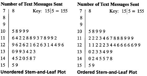
• Stem-and-Leaf Plot: Separates each data value into a "stem" and a "leaf," preserving original data values and showing distribution shape.

• Dot Plot: Plots each data entry as a point above a horizontal axis, useful for small data sets.

• Pie Chart: Represents categories as sectors of a circle, with area proportional to frequency.

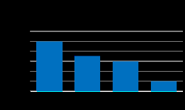
• Pareto Chart: A vertical bar graph with bars in decreasing order of frequency, used for qualitative data.

• Scatter Plot: Graphs paired data sets as points in a coordinate plane, showing relationships between two quantitative variables.

• Time Series Chart: Plots quantitative data measured at regular intervals over time.

Example: Stem-and-leaf plot for text messages sent by college dormitory residents.

Example: Pareto chart for qualitative data.

Measures of Central Tendency

Measures of central tendency describe a typical or central value in a data set. The most common are mean, median, and mode.

• Mean (Average): The sum of all data entries divided by the number of entries.

  • Population mean: $\mu = \frac{\sum x}{N}$

  • Sample mean: $\bar{x} = \frac{\sum x}{n}$

• Median: The middle value in an ordered data set. If the number of entries is odd, it is the middle entry; if even, it is the mean of the two middle entries.

• Mode: The value that occurs most frequently. If no value repeats, there is no mode; if two values repeat most often, the set is bimodal.

Example: Calculating mean, median, and mode for flight prices.

• Mean: $\bar{x} = \frac{3695}{7} \approx 527.9$

• Median: $427$ (middle value in ordered list)

• Mode: $397$ (value occurring twice)

Example: Mode for qualitative data (political party with highest frequency).

Comparing Mean, Median, and Mode

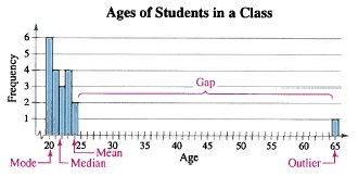
Each measure has advantages and disadvantages. The mean uses all data but is sensitive to outliers. The median is robust to outliers. The mode may not always represent a typical value.

Example: Ages in a class with an outlier.

Weighted Mean

The weighted mean accounts for varying importance (weights) of data entries. Calculated as $\bar{x} = \frac{\sum (x \cdot w)}{\sum w}$, where $w$ is the weight of each entry $x$.

Mean of Grouped Data

The mean of a frequency distribution is approximated by $\bar{x} = \frac{\sum (x \cdot f)}{n}$, where $x$ is the class midpoint and $f$ is the class frequency.

The Shape of Distributions

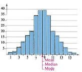
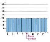
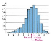
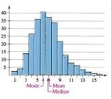
Distributions can be classified by their shape, which affects the relationship between mean, median, and mode.

• Symmetric Distribution: The halves of the graph are mirror images. Mean, median, and mode are equal.

• Uniform Distribution: All classes have equal frequencies. Mean and median are equal.

• Skewed Left (Negatively Skewed): The tail extends to the left. Mean is less than median.

• Skewed Right (Positively Skewed): The tail extends to the right. Mean is greater than median.

Additional info: These notes cover the essential concepts and graphical methods for descriptive statistics, including frequency distributions, histograms, polygons, ogives, stem-and-leaf plots, dot plots, pie charts, Pareto charts, scatter plots, time series charts, and measures of central tendency. The classification of distribution shapes is also included, with visual examples.