Descriptive Statistics: Measures of Center and Data Distributions

Descriptive Statistics

Overview of Descriptive and Inferential Statistics

Statistics is divided into two main branches: descriptive statistics and inferential statistics. Descriptive statistics focus on summarizing and describing the main features of a data set, such as its center and variability. Inferential statistics use data from a sample to make generalizations or predictions about a larger population, including hypothesis testing and estimation.

• Descriptive statistics: Summarize data using measures of center, variation, and graphical displays.

• Inferential statistics: Draw conclusions about populations based on sample data.

Populations, Samples, Parameters, and Statistics

Understanding the difference between populations and samples is fundamental in statistics. Key terms include:

• Population: The entire group of individuals or items of interest.

• Sample: A subset of the population selected for analysis.

• Parameter: A numerical value that describes a characteristic of a population.

• Statistic: A numerical value that describes a characteristic of a sample.

Good sampling methods, such as simple random sampling and stratified sampling, help ensure that the sample accurately represents the population.

Measures of Center

Introduction to Measures of Center

Measures of center are values that describe the central or typical value in a data set. The most common measures are the mean, median, mode, and midrange.

Mean (Arithmetic Mean)

The mean is the sum of all data values divided by the number of values. It is commonly referred to as the "average" and is sensitive to extreme values (outliers).

• Sample mean: Denoted as $x\bar{\ }$

• Population mean: Denoted as $\mu$

Formula for the mean:

$x\bar{\ } = \frac{\sum x}{n}$

Example: Find the mean of the data set: 22, 22, 26, 24, 23.

$x\bar{\ } = \frac{22+22+26+24+23}{5} = \frac{117}{5} = 23.4$

• Advantages: Uses all data values; sample means vary less than other measures.

• Disadvantages: Not resistant to outliers; a single extreme value can affect it dramatically.

Median

The median is the middle value when the data are arranged in order. It is a resistant measure of center, meaning it is not affected much by extreme values.

• If the number of data values is odd, the median is the exact middle value.

• If the number of data values is even, the median is the mean of the two middle values.

Example: Data: 0.42, 0.48, 0.66, 0.73, 1.10, 1.10, 5.40 (odd number of values). Median is 0.73. Data: 0.42, 0.48, 0.73, 1.10, 1.10, 5.40 (even number of values). Median is $(0.73 + 1.10)/2 = 0.915$.

Mode

The mode is the value that occurs with the greatest frequency in a data set. A data set may have one mode (unimodal), more than one mode (bimodal or multimodal), or no mode if all values are unique. The mode is the only measure of central tendency that can be used with nominal data.

• Bimodal: Two values occur with the same highest frequency.

• Multimodal: More than two values occur with the same highest frequency.

• No mode: No value is repeated.

Example: Data: 5.40, 1.10, 0.42, 0.73, 0.48, 1.10 → Mode is 1.10 Data: 27, 27, 27, 55, 55, 55, 88, 88, 99 → Bimodal (27 & 55) Data: 1, 2, 3, 6, 7, 8, 9, 10 → No mode

Midrange

The midrange is the value midway between the maximum and minimum values in the data set. It is calculated as:

$\text{Midrange} = \frac{\text{Maximum value} + \text{Minimum value}}{2}$

The midrange is sensitive to extreme values and is rarely used as the sole measure of center.

Estimating the Mean from a Frequency Distribution

When data are grouped into classes, the mean can be estimated by assuming all values in a class are equal to the class midpoint. The formula is:

$x\bar{\ } = \frac{\sum (f \cdot x)}{\sum f}$

• f: Frequency of each class

• x: Class midpoint

Example: Estimating the mean from IQ scores:

IQ Score	Frequency (f)	Class Midpoint (x)	f · x
50-69	2	59.5	119.0
70-89	33	79.5	2623.5
90-109	35	99.5	3482.5
110-129	7	119.5	836.5
130-149	1	139.5	139.5
Totals	78		7201.0

Estimated mean: $x\bar{\ } \approx \frac{7201.0}{78} = 92.32$

Weighted Mean

A weighted mean is used when data values are assigned different weights. The formula is:

$x\bar{\ } = \frac{\sum (w \cdot x)}{\sum w}$

• w: Weight assigned to each value x

Example: Calculating a student's GPA: Swahili: A (3 credits), Intro Stats: A (4 credits), Chemistry: B (3 credits), History: C (3 credits), Biology: F (1 credit) Quality points: A=4, B=3, C=2, F=0

Weighted mean: $x\bar{\ } = \frac{(3 \times 4) + (4 \times 4) + (3 \times 3) + (3 \times 2) + (1 \times 0)}{3+4+3+3+1} = \frac{37}{14} \approx 3.07$

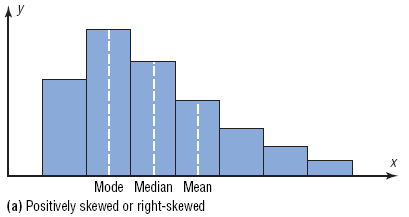
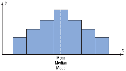
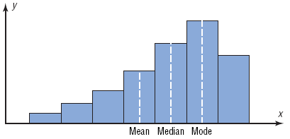
Comparing Measures of Center in Different Distributions

The relationship between the mean, median, and mode depends on the shape of the data distribution:

• Positively skewed (right-skewed): Mean > Median > Mode

• Symmetric: Mean = Median = Mode

• Negatively skewed (left-skewed): Mean < Median < Mode

Choosing the Best Measure of Center

Guidelines for selecting the most appropriate measure of center:

• Use the mean for symmetric distributions without outliers.

• Use the median for skewed distributions or when outliers are present.

• Use the mode for categorical (nominal) data.

• The midrange is rarely used due to its sensitivity to extremes.

Example: For the monthly number of surveys: 1, 8, 10, 15, 16, 22, 131, 20, 17, 15, 15, 5, the mean is affected by the outlier (131), so the median may be a better measure of center.