Descriptive Statistics: Measures of Center and Spread

Descriptive Statistics

Introduction to Descriptive Statistics

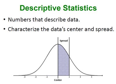
Descriptive statistics involve numbers that summarize and describe the main features of a data set. These statistics help to characterize the data’s center and spread, providing a foundation for further statistical analysis.

Statistical Notation

Understanding statistical notation is essential for interpreting formulas and calculations in statistics:

• ∑ - Denotes the sum of a set of values.

• x - Represents individual values in a data set.

• n - The number of values in a sample (sample size).

• N - The number of values in a population (population size).

Population Size vs. Sample Size

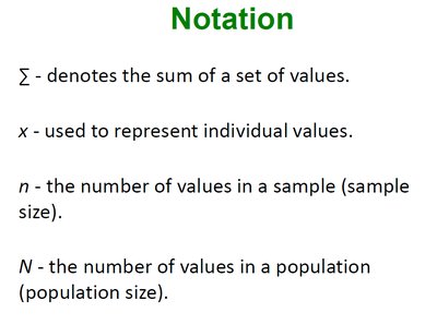
In statistics, it is important to distinguish between the population (the entire group of interest) and a sample (a subset of the population). For example, if a study involves all 50 states but only 10 are selected for analysis, the population size is 50 and the sample size is 10.

Measures of Center

Overview of Measures of Center

Measures of center describe the central or typical value in a data set. The most common measures are the mean, median, mode, and midrange.

Mean

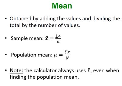
The mean is calculated by adding all values and dividing by the number of values. It is the most commonly used measure of center.

• Sample mean: $\bar{x} = \frac{\sum x}{n}$

• Population mean: $\mu = \frac{\sum x}{N}$

• Note: Calculators typically use $\bar{x}$ for both sample and population means.

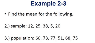
Example: Calculating the Mean

• Sample: 12, 25, 38, 5, 20

• Population: 60, 73, 77, 51, 68, 75

Calculator Notation for Descriptive Statistics

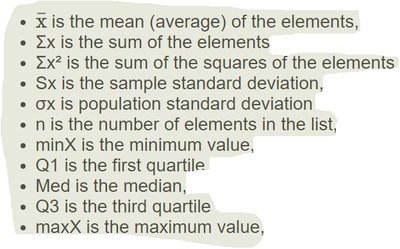
Common calculator outputs for descriptive statistics include:

• $\bar{x}$: Mean (average) of the elements

• $\sum x$: Sum of the elements

• $\sum x^2$: Sum of the squares of the elements

• $Sx$: Sample standard deviation

• $\sigma x$: Population standard deviation

• minX: Minimum value

• Q1: First quartile

• Med: Median

• Q3: Third quartile

• maxX: Maximum value

Mean of Grouped Data

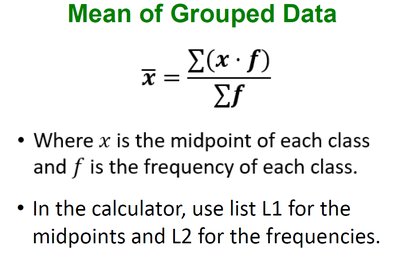
For grouped data, the mean is calculated using class midpoints and frequencies:

• Formula: $\bar{x} = \frac{\sum (x \cdot f)}{\sum f}$

• Where x is the midpoint of each class and f is the frequency of each class.

• In calculators, use one list for midpoints and another for frequencies.

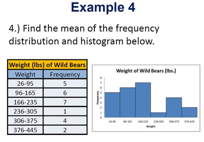
Example: Mean of a Frequency Distribution

Weight (lbs)	Frequency
26-95	5
96-165	6
166-235	7
236-305	4
306-375	4
376-445	2

Weighted Mean

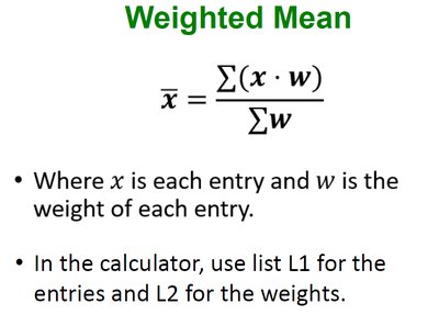
The weighted mean is used when different values contribute unequally to the average. It is calculated as:

• Formula: $\bar{x} = \frac{\sum (x \cdot w)}{\sum w}$

• Where x is each entry and w is the weight of each entry.

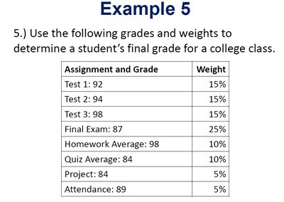
Example: Weighted Mean for Grades

Assignment and Grade	Weight
Test 1: 92	15%
Test 2: 94	15%
Test 3: 98	15%
Final Exam: 87	25%
Homework Average: 98	10%
Quiz Average: 84	10%
Project: 84	5%
Attendance: 89	5%

Resistance of the Mean

The mean is sensitive to extreme values (outliers) and is not a resistant measure of center. For example, a single very low or high value can significantly affect the mean.

Median

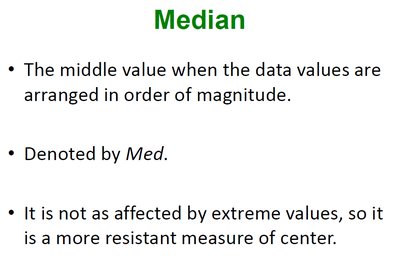
The median is the middle value when the data are arranged in order. It is denoted by Med and is more resistant to extreme values than the mean.

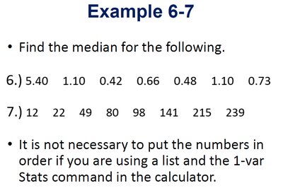
Example: Finding the Median

• 6.) 5.40, 1.10, 0.42, 0.66, 0.48, 1.10, 0.73

• 7.) 12, 22, 49, 80, 98, 141, 215, 239

Shape of the Distribution

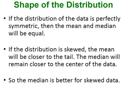
The relationship between the mean and median can indicate the shape of the data distribution:

• If the distribution is symmetric, the mean and median are equal.

• If the distribution is skewed, the mean is pulled toward the tail, while the median remains closer to the center.

• The median is preferred for skewed data.

Example: Comparing Mean and Median

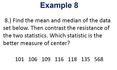
• Data: 101, 106, 109, 116, 118, 135, 568

• Find the mean and median, and discuss which is a better measure of center given the presence of an outlier (568).

Mode and Modal Class

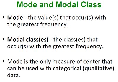
The mode is the value(s) that occur most frequently in a data set. The modal class is the class interval with the highest frequency in grouped data. Mode is the only measure of center that can be used with categorical (qualitative) data.

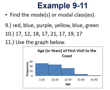
Example: Finding the Mode

• 9.) red, blue, purple, yellow, blue, green

• 10.) 17, 12, 18, 17, 21, 17, 19, 17

• 11.) Use the provided graph to determine the modal class.

Numbers of Modes

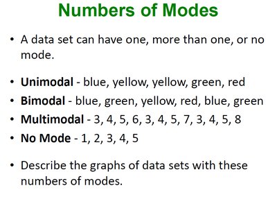
A data set can have one, more than one, or no mode:

• Unimodal: One mode (e.g., blue, yellow, yellow, green, red)

• Bimodal: Two modes (e.g., blue, green, yellow, red, blue, green)

• Multimodal: More than two modes (e.g., 3, 4, 5, 6, 3, 4, 5, 7, 3, 4, 5, 8)

• No Mode: No value repeats (e.g., 1, 2, 3, 4, 5)

Midrange

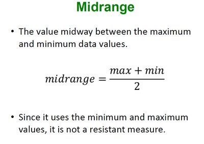
The midrange is the value midway between the maximum and minimum data values. It is calculated as:

$midrange = \frac{max + min}{2}$

Since it uses only the minimum and maximum values, the midrange is not a resistant measure.

Example: Calculating the Midrange

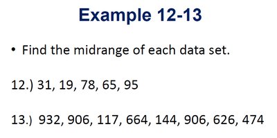
• 12.) 31, 19, 78, 65, 95

• 13.) 932, 906, 117, 664, 144, 906, 626, 474

Measures of Spread

Overview of Measures of Spread

Measures of spread describe the variation or dispersion in a data set. Common measures include the range, standard deviation, and variance.

Additional info: Measures of spread are essential for understanding how much the data values differ from the center. The range is the difference between the maximum and minimum values, the variance measures the average squared deviation from the mean, and the standard deviation is the square root of the variance.