Descriptive Statistics: Measures of Central Tendency

Descriptive Statistics

Measures of Central Tendency

Measures of central tendency are statistical values that represent a typical or central entry of a data set. They are fundamental for summarizing and understanding data distributions. The most common measures are mean, median, and mode.

• Mean: The arithmetic average, calculated as the sum of all data entries divided by the number of entries.

• Median: The middle value in an ordered data set, dividing it into two equal parts.

• Mode: The value(s) that occur most frequently in the data set.

Mean (Average)

The mean is a widely used measure of central tendency. It is calculated using the following formulas:

• Population Mean: $\mu = \frac{\sum x}{N}$

• Sample Mean: $\bar{x} = \frac{\sum x}{n}$

Example: For the sample weights 274, 235, 223, 268, 290, 285, 235, the mean is approximately 258.6 pounds.

Median

The median is the value that lies in the middle of an ordered data set. It is less affected by outliers than the mean.

• If the number of entries is odd, the median is the middle entry.

• If the number of entries is even, the median is the mean of the two middle entries.

Example: For the ordered weights 223, 235, 235, 268, 274, 285, 290, the median is 268 pounds.

Mode

The mode is the data entry that occurs with the greatest frequency. Data sets can be:

• Unimodal: One mode

• Bimodal: Two modes

• Multimodal: Three or more modes

• No mode: No repeated entries or more than three entries with the same frequency

Example: In the weights 223, 235, 235, 268, 274, 285, 290, the mode is 235 pounds.

Comparing Mean, Median, and Mode

All three measures describe a typical entry, but each has advantages and disadvantages:

• Mean: Reliable as it uses all data, but sensitive to outliers.

• Median: Robust against outliers and skewed data.

• Mode: Useful for categorical data and identifying the most frequent value.

Example: In a class with ages: mean = 23.8 years, median = 20.5 years, mode = 20 years. The mean is influenced by an outlier (age 65), so the median best describes the typical age.

When to Use Mean vs. Median

Choosing between mean and median depends on the data distribution:

• Use the mean: When data are symmetric and have no outliers.

• Use the median: When data are skewed or contain outliers.

Weighted Mean

The weighted mean accounts for varying weights in the data entries. It is calculated as:

• $\bar{x} = \frac{\sum w x}{\sum w}$

Example: Mark’s GPA is calculated as a weighted mean based on grade points and credit hours.

Mean of Grouped Data

For frequency distributions, the mean is estimated using class midpoints and frequencies:

• $\bar{x} = \frac{\sum x f}{\sum f}$

Example: For cell phone screen times grouped by frequency, the estimated mean is 287.7 minutes.

The Shape of Distributions

The shape of a distribution affects which measure of central tendency is most appropriate:

• Symmetric Distribution: Mirror image halves; mean ≈ median ≈ mode.

• Uniform Distribution: All classes have equal frequencies; symmetric.

• Normal Distribution: Symmetrical and unimodal; mean = median = mode.

• Skewed Left: Tail extends to the left; mean < median.

• Skewed Right: Tail extends to the right; mean > median.

Using StatCrunch to Find Mean and Median

Statistical software like StatCrunch can be used to calculate mean and median efficiently. Enter data under the variable column and use the summary statistics function to compute these measures.

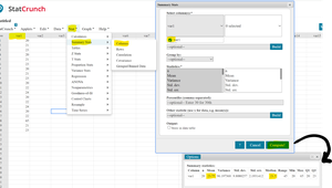
Additional info: StatCrunch is a tool for performing statistical calculations and visualizations, useful for both descriptive and inferential statistics.