Descriptive Statistics: Measures of Variation

Measures of Variation

Introduction

Measures of variation are essential in statistics for describing how data values are spread or dispersed around the center of a data set. Understanding variation helps us interpret the consistency, reliability, and risk associated with data.

• Range

• Standard Deviation

• Variance

• Coefficient of Variation

• Quartiles (covered in Section 2.5)

Range

The range is the simplest measure of variation, calculated as the difference between the maximum and minimum values in a data set. It provides a quick sense of the spread but is sensitive to outliers.

• Formula: $\text{Range} = \text{Maximum value} - \text{Minimum value}$

• Example: Two corporations each hired 10 graduates with identical mean and median salaries, but Corporation A had a range of $10,000 and Corporation B had a range of $35,000, illustrating significant differences in spread despite similar centers.

Standard Deviation and Variance

Standard deviation quantifies the typical distance each data point is from the mean. Variance is the average of the squared differences from the mean. These measures are more robust than the range and are fundamental for statistical analysis.

• Sample Variance: $s^2 = \frac{\sum (x_i - \bar{x})^2}{n-1}$

• Sample Standard Deviation: $s = \sqrt{\frac{\sum (x_i - \bar{x})^2}{n-1}}$

• Population Variance: $\sigma^2 = \frac{\sum (x_i - \mu)^2}{N}$

• Population Standard Deviation: $\sigma = \sqrt{\frac{\sum (x_i - \mu)^2}{N}}$

• Interpretation: A small standard deviation indicates values are close to the mean (consistent), while a large standard deviation indicates greater spread (inconsistent).

• Example: Recovery times for concussed football players: sample standard deviation calculated as approximately 2.2 days.

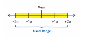
Interpreting Standard Deviation: Usual Range

Standard deviation helps identify the usual range of values. Values outside this range may be considered unusual and warrant further investigation.

• Usual Range: Typically, values within two standard deviations of the mean are considered usual.

• Formula: $\text{Usual Range} = [\text{Mean} - 2\sigma, \text{Mean} + 2\sigma]$

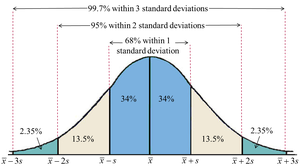
Empirical Rule (68–95–99.7 Rule)

The Empirical Rule applies to data sets that are approximately normal (symmetrical and unimodal). It describes the percentage of data within 1, 2, and 3 standard deviations of the mean.

• About 68% of data falls within 1 standard deviation ($\mu \pm \sigma$)

• About 95% within 2 standard deviations ($\mu \pm 2\sigma$)

• About 99.7% within 3 standard deviations ($\mu \pm 3\sigma$)

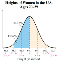
Example: Heights of Women in the U.S. (Ages 20–29)

For heights, the Empirical Rule can be used to estimate the proportion of women within certain height ranges.

• About 47.72% of women are between 58.9 and 64.1 inches tall.

Standard Deviation for Grouped Data

When data are grouped into classes (frequency distributions), the sample mean and standard deviation can be estimated using class midpoints.

• Procedure: Use the midpoint of each class and the frequency to estimate statistics.

• Example: Number of children in U.S. families, price ranges of homes.

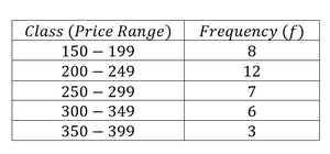
Example Table: Price Ranges of Homes

Class (Price Range)	Frequency (f)
150 – 199	8
200 – 249	12
250 – 299	7
300 – 349	6
350 – 399	3

Summarizing Data: Center and Spread

Both center and spread are needed to fully describe a data set. The choice of summary statistics depends on the shape of the distribution.

• Symmetric, unimodal data: Use mean and standard deviation.

• Skewed data: Use median and interquartile range (IQR).

Coefficient of Variation (CV)

The coefficient of variation (CV) expresses the standard deviation as a percentage of the mean, allowing comparison of variability across data sets with different units or scales.

• Formula for population: $\text{CV} = \frac{\sigma}{\mu} \times 100\%$

• Formula for sample: $\text{CV} = \frac{s}{\bar{x}} \times 100\%$

• Application: Useful for comparing GPA and income, heights and weights, etc., where direct comparison of standard deviations is not meaningful.

Example: Heights and Weights of a Basketball Team

The table below shows the heights and weights of team members. The CV allows us to compare the relative variability of these two measurements.

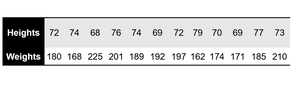
Statistic	Heights	Weights
Mean (μ)	72.8 inches	187.8 pounds
Standard Deviation (σ)	3.3 inches	17.7 pounds
Coefficient of Variation (CV)	4.5%	9.4%

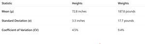
Interpretation: Although the standard deviation for weights is numerically larger, the CV shows that weights have greater relative variability compared to heights.

Conclusion

Measures of variation are crucial for understanding the spread and consistency of data. Range, standard deviation, variance, and coefficient of variation each provide unique insights, and their appropriate use depends on the context and nature of the data set.