Descriptive Statistics: Measures of Variation and Position

Measures of Variation

Range

The range is the simplest measure of variation in a data set. It is calculated as the difference between the maximum and minimum values in a quantitative data set.

• Formula: Range = (Maximum value) – (Minimum value)

• Example: For starting salaries: 41, 38, 39, 45, 47, 41, 44, 41, 37, 42, the range is 47 – 37 = 10 ($10,000).

Deviation, Variance, and Standard Deviation

These measures describe how data entries deviate from the mean, providing insight into the spread of the data.

• Deviation: The difference between a data entry and the mean.

  • Population: deviation of x = x – μ

  • Sample: deviation of x = x – \bar{x}

• Population Variance: The average of the squared deviations from the mean.

  • Formula: $\sigma^2 = \frac{\sum (x - \mu)^2}{N}$

• Population Standard Deviation: The square root of the variance.

  • Formula: $\sigma = \sqrt{\frac{\sum (x - \mu)^2}{N}}$

• Sample Variance: Uses n-1 in the denominator to correct for bias.

  • Formula: $s^2 = \frac{\sum (x - \bar{x})^2}{n-1}$

• Sample Standard Deviation: The square root of the sample variance.

  • Formula: $s = \sqrt{\frac{\sum (x - \bar{x})^2}{n-1}}$

• Example: For the starting salaries, the sample standard deviation is about 3.1 ($3,100).

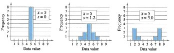
Interpreting Standard Deviation

The standard deviation measures the typical amount an entry deviates from the mean. Larger standard deviations indicate more spread out data.

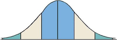
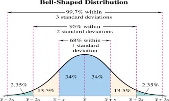
Empirical Rule (68–95–99.7 Rule)

For data with a symmetric, bell-shaped distribution, the Empirical Rule describes the proportion of data within 1, 2, and 3 standard deviations of the mean:

• About 68% within 1 standard deviation

• About 95% within 2 standard deviations

• About 99.7% within 3 standard deviations

Chebychev’s Theorem

Chebychev’s Theorem applies to any data set, regardless of distribution shape. It states that at least $1 - \frac{1}{k^2}$ of the data lies within k standard deviations of the mean (for k > 1).

• For k = 2: At least 75% within 2 standard deviations

• For k = 3: At least 88.9% within 3 standard deviations

Standard Deviation for Grouped Data

When data is grouped into classes, use class midpoints and frequencies to estimate the sample mean and standard deviation.

• Formula: $s = \sqrt{\frac{\sum (x - \bar{x})^2 f}{n-1}}$ where n = total frequency

• Example: For 50 households, the sample mean number of children is about 1.8, and the standard deviation is about 1.7.

Coefficient of Variation (CV)

The coefficient of variation expresses the standard deviation as a percentage of the mean, allowing comparison of variability between different data sets.

• Population: $CV = \frac{\sigma}{\mu} \times 100\%$

• Sample: $CV = \frac{s}{\bar{x}} \times 100\%$

• Example: Comparing heights and weights of a basketball team:

Heights	Weights
72	180
74	168
68	225
76	201
74	189
69	192
72	197
79	162
70	174
69	171
77	185
73	210

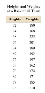
• Heights: CV ≈ 4.5%

• Weights: CV ≈ 9.4%

• Interpretation: Weights are more variable than heights.

Measures of Position

Quartiles

Quartiles are fractiles that divide an ordered data set into four equal parts:

• Q1: First quartile, about 25% of data below

• Q2: Second quartile (median), about 50% below

• Q3: Third quartile, about 75% below

• Example: For nuclear power plants in 15 countries, Q1 = 10, Q2 = 18, Q3 = 31.

Interquartile Range (IQR)

The interquartile range measures the spread of the middle 50% of the data:

• Formula: IQR = Q3 – Q1

• Example: IQR = 31 – 10 = 21

Box-and-Whisker Plot

A box-and-whisker plot is a graphical tool that displays the five-number summary (minimum, Q1, median, Q3, maximum) and highlights the spread and possible outliers in a data set.

• Steps: Find five-number summary, construct scale, plot points, draw box from Q1 to Q3, mark median, draw whiskers to min and max.

• Interpretation: The length of whiskers can indicate outliers.

Percentiles and Other Fractiles

Fractiles partition data into equal parts:

Type	Divides Data Into	Symbols
Quartiles	4 parts	Q1, Q2, Q3
Deciles	10 parts	D1, D2, ..., D9
Percentiles	100 parts	P1, P2, ..., P99

• Example: SAT scores and percentiles.

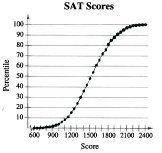
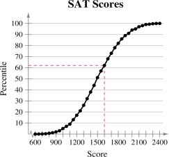
• 62nd percentile corresponds to a score of 1600: 62% of students scored 1600 or less.

Standard Score (z-score)

The z-score indicates how many standard deviations a value is from the mean. It allows comparison across different data sets.

• Formula: $z = \frac{x - \mu}{\sigma}$

• Example: Heath Ledger's z-score for age at Oscar win: $z \approx -1.49$; Penelope Cruz: $z \approx -0.42$

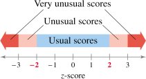
• Interpretation: Scores between -2 and 2 are considered usual; outside this range are unusual or very unusual.

Summary

• Found the range, variance, and standard deviation for populations and samples

• Used Empirical Rule and Chebychev’s Theorem to interpret standard deviation

• Approximated sample standard deviation for grouped data

• Used coefficient of variation to compare variation in different data sets

• Found quartiles, interquartile range, and represented data with box-and-whisker plots

• Interpreted percentiles and z-scores for measures of position