Descriptive Statistics: Organizing and Summarizing Data

Chapter 2: Descriptive Statistics

2.1 Organizing Qualitative Data

Qualitative (or categorical) data allows for classification of individuals based on attributes or characteristics. Organizing such data involves creating frequency distributions and visual representations to summarize the data effectively.

• Frequency Distribution: A table that lists categories and the number of occurrences (frequency) for each category.

• Relative Frequency: The proportion of observations in each category, calculated as: $\text{Relative Frequency} = \frac{\text{Frequency}}{\text{Total Number of Observations}}$

• Visual Representations: Bar graphs and pie charts are commonly used to display qualitative data.

Example: Frequency Distribution of Injury Location

A physical therapist records the body part requiring rehabilitation for 30 patients. The frequency distribution is constructed as follows:

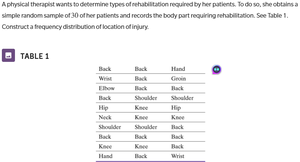
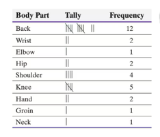
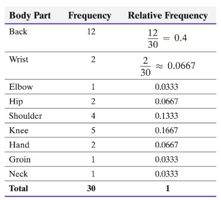
• Check: The sum of frequencies equals the total number of observations (30). The sum of relative frequencies equals 1.

Bar Graphs and Pie Charts

• Bar Graph: Categories are labeled on one axis, and frequency or relative frequency on the other. Rectangles of equal width represent each category, with height proportional to frequency.

• Pie Chart: A circle divided into sectors, each representing a category. The area of each sector is proportional to the category's frequency.

2.2 Organizing Quantitative Data

Quantitative data can be discrete (countable values) or continuous (measured values). Organizing quantitative data involves creating frequency distributions, histograms, and other visual displays.

• Discrete Data: Categories (classes) are the distinct values observed. Frequency and relative frequency distributions are constructed, and bar graphs or histograms are used for visualization.

• Continuous Data: Data is grouped into intervals (classes). Frequency and relative frequency distributions are constructed, and histograms are used for visualization.

Constructing Frequency Distribution for Continuous Data

• Step 1: Write the lowest value as the first class lower limit.

• Step 2: Add the class width to calculate subsequent lower limits.

• Step 3: Calculate upper limits for each class.

• Step 4: Tally the data into classes and record frequencies.

• Step 5: Calculate relative frequencies.

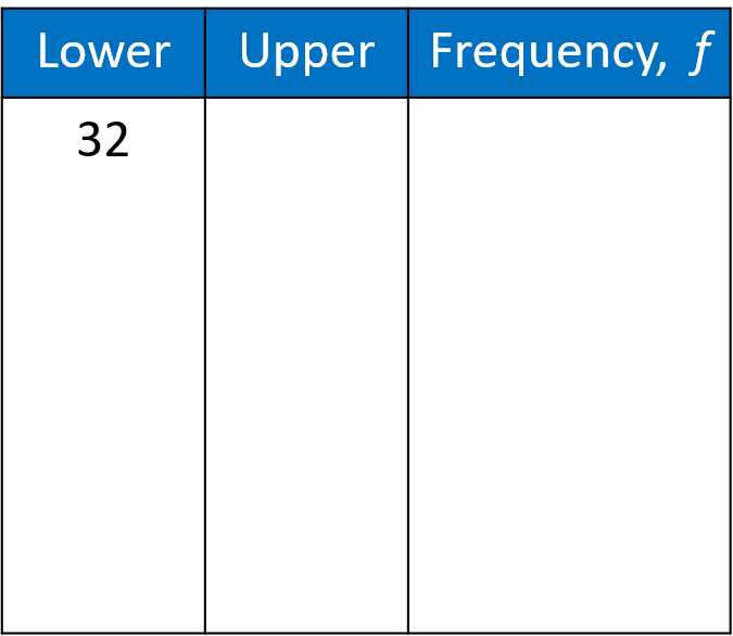
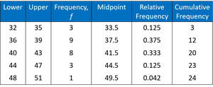
Example: Organizing Exit Velocity Data

Given a sample of exit velocities from home runs, histograms are constructed using different class widths to summarize the data.

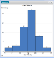
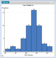
• Comparison: The choice of class width affects the summary and interpretation of the data. Smaller class widths provide more detail, while larger class widths offer a broader overview.

2.3 Shape of a Distribution

The shape of a distribution describes how data values are spread and can be classified as symmetric, uniform, skewed left, or skewed right.

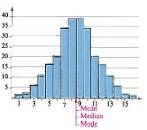
• Symmetric (Bell-Shaped) Distribution: The halves of the graph are mirror images. Mean, median, and mode are approximately equal.

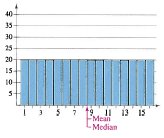
• Uniform Distribution: All classes have equal or nearly equal frequencies. The distribution is symmetric.

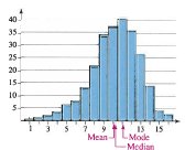
• Skewed Left (Negatively Skewed): The tail extends to the left. Most data is to the right of the median. Mean is less than the median.

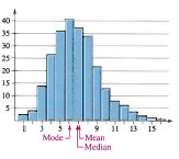
• Skewed Right (Positively Skewed): The tail extends to the right. Most data is to the left of the median. Mean is greater than the median.

2.4 Additional Displays of Quantitative Data

• Dot Plot: Each observation is placed in order, and a dot is drawn above each value for every occurrence.

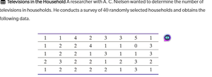
• Stem-and-Leaf Plot: Each number is separated into a stem (all but the last digit) and a leaf (last digit). This display is similar to a histogram but retains original data values.

Example: Constructing a Stem-and-Leaf Plot

1. Sort data from lowest to highest.

2. Create the stem-and-leaf plot by listing stems and attaching leaves.

Summary: Organizing and summarizing data using frequency distributions, bar graphs, pie charts, histograms, dot plots, and stem-and-leaf plots provides a foundation for understanding the characteristics and patterns within a dataset.

HTML Table Example: Frequency Distribution for Injury Location

Body Part	Frequency	Relative Frequency
Back	12	0.4
Wrist	2	0.0667
Elbow	1	0.0333
Hip	2	0.0667
Shoulder	4	0.1333
Knee	5	0.1667
Hand	2	0.0667
Groin	1	0.0333
Neck	1	0.0333
Total	30	1

HTML Table Example: Frequency Distribution for Continuous Data

Lower	Upper	Frequency, f	Midpoint	Relative Frequency	Cumulative Frequency
32	35	3	33.5	0.125	3
36	39	9	37.5	0.375	12
40	43	8	41.5	0.333	20
44	47	3	44.5	0.125	23
48	51	1	49.5	0.042	24

Additional info: Academic context was added to clarify the steps for constructing frequency distributions, the interpretation of histograms, and the classification of distribution shapes.