Discrete and Binomial Probability Distributions: Concepts, Formulas, and Applications

Random Variables and Probability Distributions

Basic Concepts of Probability Distribution

A random variable is a variable whose values are determined by chance. Random variables are fundamental in statistics for modeling outcomes of random processes.

• Discrete Random Variable: Takes on a finite or countable number of values (e.g., number of heads in coin tosses, number of children in a family).

• Continuous Random Variable: Can take any value within a range, including decimals and fractions (e.g., weight, temperature).

A probability distribution lists all possible outcomes of a random variable and their corresponding probabilities. These probabilities can be determined theoretically or by observation and are often presented in tables, graphs, or formulas.

Requirements for Probability Distributions

• There is a numerical random variable, x, with associated probabilities.

• The sum of all probabilities must be 1.

• Each probability value must be between 0 and 1, inclusive.

Discrete Probability Distributions

Definition and Examples

A discrete probability distribution consists of the values a discrete random variable can assume and their corresponding probabilities.

• Example 1: Coin Toss – Tossing two coins, let X be the number of heads. Possible outcomes: 0, 1, or 2 heads.

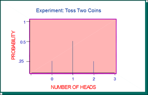
• Example 2: Number of Girls in Two Births – Possible outcomes: 0, 1, or 2 girls.

Probability Distribution Table

Probability distributions are often represented in tables. For example, the probability distribution for the number of girls in two births:

Number of Girls (x)	Probability P(x)
0	0.25
1	0.50
2	0.25

Additional info: Probabilities are calculated based on the assumption that each child is equally likely to be a girl or a boy.

Probability Histogram

A probability histogram visually represents the probability distribution of a discrete random variable.

Formulas for Discrete Probability Distributions

• Mean (Expected Value): $\mu = \sum [x \cdot P(x)]$

• Variance: $\sigma^2 = \sum [(x - \mu)^2 \cdot P(x)]$

• Variance (Shortcut): $\sigma^2 = \sum [x^2 \cdot P(x)] - \mu^2$

• Standard Deviation: $\sigma = \sqrt{\sigma^2}$

Identifying Unusual Results: Range Rule of Thumb

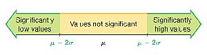
The range rule of thumb helps identify significantly low or high values in a probability distribution:

• Significantly low values: $\mu - 2\sigma$ or lower

• Significantly high values: $\mu + 2\sigma$ or higher

• Values not significant: Between $\mu - 2\sigma$ and $\mu + 2\sigma$

Expected Value

Definition and Calculation

The expected value (E) of a discrete random variable is the mean value of its outcomes, calculated as:

• $E = \sum [x \cdot P(x)]$

This value represents the long-term average if the experiment is repeated many times.

Binomial Probability Distribution

Definition and Requirements

A binomial probability distribution arises from a procedure that meets these requirements:

• Fixed number of trials (n).

• Each trial is independent.

• Each trial has only two possible outcomes: success (S) or failure (F).

• The probability of success (p) remains the same for each trial.

Notation

• n: Number of trials

• x: Number of successes in n trials

• p: Probability of success in one trial

• q: Probability of failure in one trial ($q = 1 - p$)

• P(x): Probability of getting exactly x successes

Binomial Probability Formula

The probability of getting exactly x successes in n independent trials is given by:

• $P(x) = \frac{n!}{x!(n-x)!} p^x q^{n-x}$

Where $n!$ denotes the factorial of n.

Methods for Calculating Binomial Probabilities

• Using the general formula for the binomial distribution

• Using binomial probability tables

• Using statistical software or calculators

Parameters of the Binomial Probability Distribution

• Mean: $\mu = np$

• Variance: $\sigma^2 = npq$

• Standard Deviation: $\sigma = \sqrt{npq}$

Range Rule of Thumb for Binomial Distributions

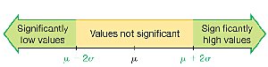
To identify significantly low or high values in a binomial distribution, use:

• Significantly low: $\mu - 2\sigma$ or lower

• Significantly high: $\mu + 2\sigma$ or higher

• Not significant: Between $\mu - 2\sigma$ and $\mu + 2\sigma$

Applications and Examples

Example: Probability of Knowing Twitter

Given a probability of 0.85 that an adult knows of Twitter, the probability of exactly 3 out of 5 adults knowing Twitter can be found using the binomial formula with n = 5, x = 3, p = 0.85, q = 0.15.

Example: Probability Table Usage

For a sample of 15 males with a 40% smoking rate, the probability that exactly 12 smoke is found using a binomial probability table: n = 15, x = 12, p = 0.4.

Example: McDonald's Recognition Rate

With a 95% recognition rate and a group of 12 adults, the mean, variance, and standard deviation for the number recognizing McDonald's are calculated as:

• Mean: $\mu = np$

• Variance: $\sigma^2 = npq$

• Standard Deviation: $\sigma = \sqrt{npq}$

The range rule of thumb is then used to determine if 12 recognitions is significantly high.

Example: Probability of Twins

If 2% of births result in twins, for a sample of 8000 births, the mean, variance, and standard deviation for the number of twin births are calculated using the binomial parameters.

Example: Teenagers with Part-Time Jobs

If 30% of teenagers have part-time jobs, and 5 are selected at random, the probability that at least 3 have part-time jobs is found using the binomial probability table.

Additional info: These examples illustrate the practical application of discrete and binomial probability distributions in real-world scenarios, such as marketing surveys, health statistics, and social research.