Discrete and Binomial Probability Distributions: Study Notes

Chapter 5: Random Variables and Probability Distributions

5.1 Discrete Random Variables

Random variables are fundamental in statistics for modeling outcomes of probability experiments numerically. They can be classified as either discrete or continuous, each with distinct properties and applications.

• Random Variable: A variable that assigns a numerical value to each outcome in a probability experiment.

• Discrete Random Variable: Takes on a countable number of distinct values (e.g., number of candies in a bag).

• Continuous Random Variable: Takes on an infinite number of possible values within a given range (e.g., mass or diameter of a candy).

Example: For a bag of M&M’s:

• Mass of each M&M: Continuous (can take any value within a range)

• Number of pieces of candy: Discrete (countable whole numbers)

• Diameter of each piece: Continuous

• Number of distinct colors: Discrete

Discrete Probability Distributions

A discrete probability distribution lists each possible value a discrete random variable can take, along with its probability. The probabilities must satisfy two rules:

• Each probability is between 0 and 1, inclusive.

• The sum of all probabilities is 1.

Example: Chuck-a-Luck game (profit from a $1 bet):

Number of Dice Matching	Profit (X)	Probability
0	-$1	0.5787
1	$1	0.3472
2	$2	0.0695
3	$3	0.0046

To verify a probability distribution, check that all probabilities are between 0 and 1 and their sum is 1.

Mean (Expected Value) of a Discrete Random Variable

The mean (or expected value) of a discrete random variable X is a measure of its long-run average value, calculated as:

$\mu = E(X) = \sum [x \cdot P(x)]$

Example: For the Chuck-a-Luck game, the mean is calculated by multiplying each profit by its probability and summing the results.

Profit (X)	Probability
-$1	0.5787
$1	0.3472
$2	0.0695
$3	0.0046

The expected value tells us the average profit (or loss) per game in the long run.

Interpretation: The mean represents the expected outcome if the experiment is repeated many times.

Standard Deviation of a Discrete Random Variable

The standard deviation measures the variability or spread of a random variable’s possible values. It is calculated as:

$\sigma = \sqrt{\sum [(x - \mu)^2 \cdot P(x)]}$

Example: For the Chuck-a-Luck game, use the probabilities and profits to compute the standard deviation, which quantifies how much the profit varies from the mean.

5.2 The Binomial Probability Distribution

The binomial distribution models the number of successes in a fixed number of independent trials, each with the same probability of success. It is widely used for yes/no type experiments.

• Each trial has two outcomes: success or failure.

• The probability of success (p) is constant for each trial.

• The trials are independent.

• The number of trials (n) is fixed.

Example: Rolling a pair of dice 10 times and counting the number of times a 7 appears is a binomial experiment (n = 10, p = probability of rolling a 7, x = number of 7’s rolled).

Computing Binomial Probabilities

The probability of getting exactly x successes in n trials is given by the binomial probability formula:

$P(X = x) = {n \choose x} p^x (1-p)^{n-x}$

Where:

• $n$ = number of trials

• $x$ = number of successes

• $p$ = probability of success on a single trial

• ${n \choose x}$ = number of combinations of n items taken x at a time

Example: If 72% of Americans would rather give up chocolate than their cell phone, in a sample of 10, the probability that exactly 8 would rather give up chocolate is calculated using the binomial formula.

Mean and Standard Deviation of a Binomial Random Variable

For a binomial random variable X with n trials and probability of success p:

• Mean: $\mu = np$

• Standard Deviation: $\sigma = \sqrt{np(1-p)}$

Example: If American Airlines flights are on time 80% of the time and 15 flights are selected, the mean and standard deviation of the number of on-time flights are:

$\mu = 15 \times 0.8 = 12$

$\sigma = \sqrt{15 \times 0.8 \times 0.2} = \sqrt{2.4} \approx 1.55$

Graphical Representation of Probability Distributions

Probability distributions can be represented graphically, with the probability values on the vertical axis. This helps visualize the likelihood of different outcomes.

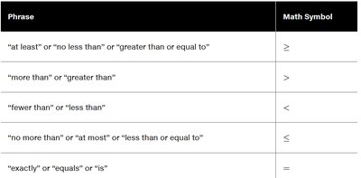
Additional info: The graphical image provided is a template for plotting probability distributions, where the y-axis represents probability values from 0 to 0.7. The table image is a useful reference for translating verbal probability statements into mathematical inequalities, which is essential for interpreting binomial probability questions.