Discrete and Continuous Random Variables, Probability Distributions, and the Normal Distribution

Discrete Random Variables

Definition and Examples

A discrete random variable is a variable whose possible values are countable and arise from the outcome of a random experiment. Examples include the number of boys in a family, the number of defective light bulbs in a box, or the number of customers arriving at a bank within a given time period. These values are finite or countably infinite and can be listed out.

• Random Variable: A numerical value generated by a random experiment.

• Discrete Random Variable: Takes on countable values (e.g., 0, 1, 2, ...).

• Continuous Random Variable: Takes on values in a continuous interval (see below).

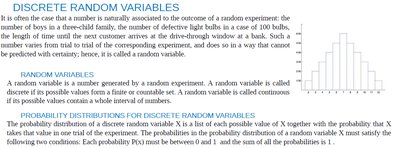
Probability Distributions for Discrete Random Variables

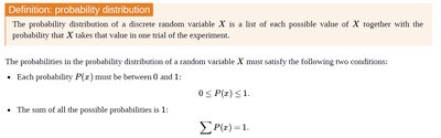
The probability distribution of a discrete random variable X is a list of each possible value of X together with the probability that X takes that value in one trial of the experiment. The probabilities must satisfy two conditions:

• Each probability P(x) must be between 0 and 1: $0 \leq P(x) \leq 1$

• The sum of all possible probabilities is 1: $\sum P(x) = 1$

Continuous Random Variables

Definition and Properties

A continuous random variable is one whose set of possible values contains a whole interval of decimal numbers. For such variables, the probability that X assumes any single particular value is zero; instead, probabilities are assigned to intervals of values.

• Examples: Heights of people, time until an event occurs, weights of objects.

• Probabilities are calculated over intervals, not at specific points.

Probability Distributions for Continuous Random Variables

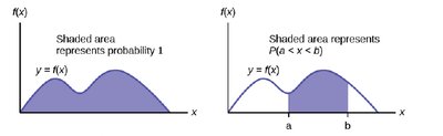
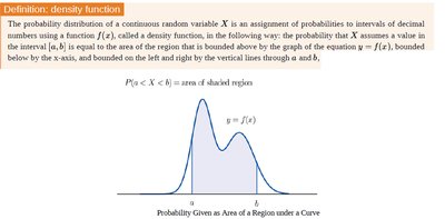
The probability distribution of a continuous random variable X is described by a density function f(x). The probability that X assumes a value in the interval [a, b] is equal to the area under the curve of f(x) from a to b:

• $P(a < X < b) = \text{Area under } f(x) \text{ from } a \text{ to } b$

• The total area under the density curve is 1.

Common Continuous Distributions

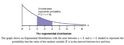
• Exponential Distribution: Models the time between events in a Poisson process. The probability that X is between two values is the area under the curve between those values.

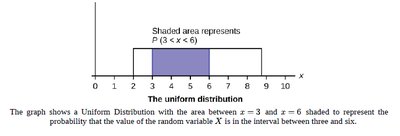
• Uniform Distribution: All intervals of the same length within the distribution's range are equally probable.

The Normal Distribution

Definition and Formula

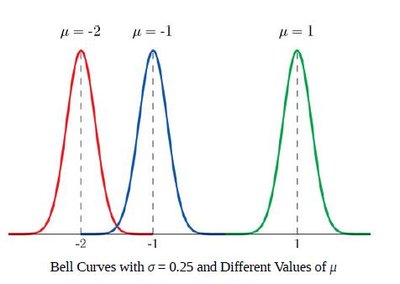
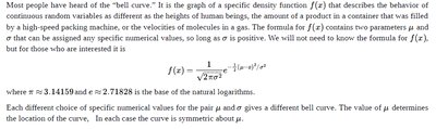
The normal distribution is a continuous probability distribution that is symmetric and bell-shaped. It is defined by two parameters: the mean (μ) and the standard deviation (σ). The probability density function is:

$f(x) = \frac{1}{\sqrt{2\pi\sigma^2}} e^{-\frac{(x-\mu)^2}{2\sigma^2}}$

• μ determines the center (location) of the curve.

• σ determines the spread (width) of the curve.

Properties of the Normal Distribution

• The curve is symmetric about the mean μ.

• The total area under the curve is 1.

• The mean, median, and mode are all equal.

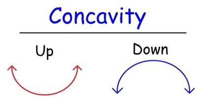
• Inflection points occur at μ ± σ, where the curve changes concavity.

The Empirical Rule (68-95-99.7 Rule)

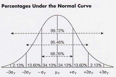
The empirical rule describes the percentage of data within certain standard deviations from the mean in a normal distribution:

• About 68% of values lie within 1 standard deviation (μ ± σ).

• About 95% of values lie within 2 standard deviations (μ ± 2σ).

• About 99.7% of values lie within 3 standard deviations (μ ± 3σ).

Interpreting Normal Curves

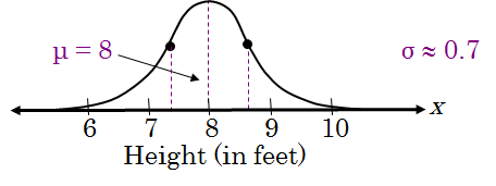
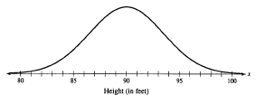
Given a normal curve, the mean is the center of symmetry, and the standard deviation can be estimated by the distance from the mean to the inflection points.

• Example: If the mean height of magnolia bushes is 8 feet and the inflection points are at 7.3 and 8.7, then σ ≈ 0.7 feet.

Standard Normal Distribution and Z-Scores

Standard Normal Distribution

The standard normal distribution is a normal distribution with mean μ = 0 and standard deviation σ = 1. Any normal random variable X can be converted to a standard normal variable Z using the transformation:

$z = \frac{x - \mu}{\sigma}$

• Z-scores measure how many standard deviations a value is from the mean.

Using the Standard Normal Table

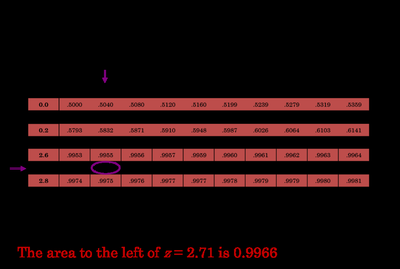
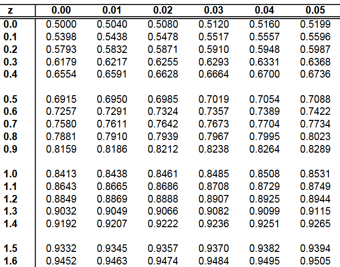
The cumulative standard normal table gives the area (probability) to the left of a given z-score. To find probabilities:

• For P(Z < z), read the table directly.

• For P(Z > z), compute 1 - P(Z < z).

• For P(a < Z < b), compute P(Z < b) - P(Z < a).

Finding Probabilities for Normal Distributions

To find the probability that a normal random variable X falls within a certain interval:

1. Convert the X values to Z-scores using $z = \frac{x - \mu}{\sigma}$.

2. Use the standard normal table to find the corresponding area (probability).

• Example: If X ~ N(500, 100), P(X < 600) = P(Z < 1) = 0.8413.

Finding Values Given Probabilities (Percentiles)

To find the value x corresponding to a given percentile (area to the left):

1. Find the z-score corresponding to the desired area using the standard normal table.

2. Transform back to the original scale: $x = \mu + z\sigma$.

• Example: For the top 5% (95th percentile), find z ≈ 1.645, then compute x.

Summary Table: Key Properties of Discrete vs. Continuous Random Variables

Property	Discrete Random Variable	Continuous Random Variable
Possible Values	Countable (finite or infinite)	Any value in an interval
Probability at a Point	P(X = x) > 0	P(X = x) = 0
Probability Calculation	Sum of probabilities	Area under density curve
Total Probability	$\sum P(x) = 1$	Total area = 1

Additional info: This guide covers foundational concepts for understanding probability distributions, including the normal distribution, which is central to inferential statistics and hypothesis testing.