5 Discrete Probability Distributions and the Binomial Distribution

Discrete Probability Distributions

Random Variables

A random variable is a quantitative variable whose values are determined by chance. Random variables link the sample space of an experiment to numerical values, allowing us to analyze outcomes mathematically.

• Discrete random variable: Takes on finite or countable values (usually integers). Examples: Number of heads when tossing a coin twice; number of TVs in a family.

• Continuous random variable: Can take on infinitely many values, often measured rather than counted. Examples: Waiting time at a doctor's office; height of a group of people; amount of rain in a city during summer.

Probability Distributions

A probability distribution describes the probability for each value of a random variable. For discrete random variables, this is often presented as a table, formula, or graph.

• The probability mass function (p.m.f.) for a discrete random variable X is denoted as f(x) or P(X = x).

• The probability distribution table has two columns: one for the values of X, and one for the corresponding probabilities.

Example: Tossing a Coin Three Times

Let X = Number of heads when tossing a coin three times. The possible values (support) are S = {0, 1, 2, 3}.

X	P(X = x)
0	1/8
1	3/8
2	3/8
3	1/8

To find the probability of getting at least 2 heads: $P(X \geq 2) = P(X = 2) + P(X = 3) = \frac{3}{8} + \frac{1}{8} = 0.5$

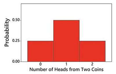
Probability Histogram

A probability histogram is similar to a relative frequency histogram, but the vertical axis shows probabilities instead of frequencies.

Requirements for a Discrete Probability Distribution

• Each probability is between 0 and 1: $0 \leq P(x) \leq 1$

• The sum of all probabilities is 1: $\sum P(x) = 1$

Tables that do not meet these requirements (e.g., negative probabilities or probabilities that do not sum to 1) are not valid probability distributions.

Identifying Discrete and Continuous Variables

Situation	Discrete	Continuous
Time to register for classes		X
Number of bad checks at a bank	X
Amount of gasoline for 200 miles		X
Number of traffic fatalities per year	X
Distance a golf ball travels		X
Number of boats on a reservoir	X
Weight before breakfast		X

Parameters of a Probability Distribution

Expected Value (Mean)

The expected value (mean) of a discrete probability distribution is the central value of the random variable:

$\mu = E[X] = \sum [x \cdot P(x)]$

Example: For the number of heads when tossing a coin twice:

X	P(X)
0	0.25
1	0.5
2	0.25

$E(X) = 0 \times 0.25 + 1 \times 0.5 + 2 \times 0.25 = 1$

Variance and Standard Deviation

• Variance: $\sigma^2 = \sum (x - \mu)^2 P(x)$ or $\sigma^2 = \sum [x^2 P(x)] - \mu^2$

• Standard deviation: $\sigma = \sqrt{\sigma^2}$

Example: For the number of heads when tossing a coin twice:

$\sigma^2 = 1.5 - 1^2 = 0.5$ $\sigma = \sqrt{0.5} = 0.707$

Binomial Probability Distribution

Bernoulli Trials

Repeated trials of an experiment are called Bernoulli trials if:

• Each trial has two possible outcomes: "Success" (S) or "Failure" (F).

• Trials are independent.

• The probability of success (p) is constant for each trial.

The probability mass function for a Bernoulli random variable X is:

$P(X = x) = \begin{cases} 1 - p & \text{if } x = 0 \\ p & \text{if } x = 1 \end{cases}$

Binomial Distribution

The binomial distribution gives the probability of x successes in n independent Bernoulli trials with probability p of success:

$P(x) = \frac{n!}{(n-x)!x!} p^x (1-p)^{n-x}$

• n = number of trials

• x = number of successes

• p = probability of success

• q = 1 - p = probability of failure

Note: The definition of "success" is arbitrary and must be consistent for both x and p.

Example: Genetics and Binomial Distribution

• Probability a child has type O blood: p = 0.25

• Number of children: n = 4

• X ~ Binomial(n = 4, p = 0.25)

Mean and Standard Deviation of Binomial Distribution

• Mean: $\mu = np$

• Variance: $\sigma^2 = np(1-p)$

• Standard deviation: $\sigma = \sqrt{np(1-p)}$

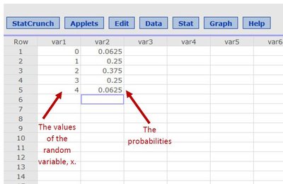
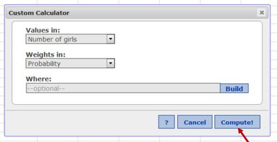
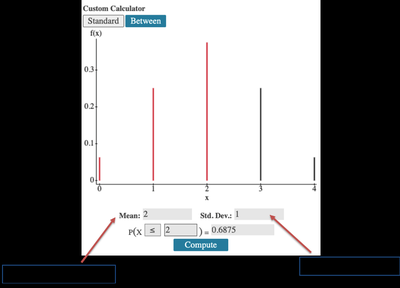
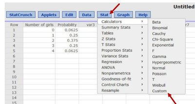
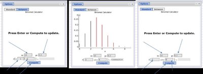
Using StatCrunch for Probability Calculations

StatCrunch can be used to compute probabilities, means, and standard deviations for custom and binomial distributions.

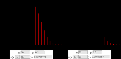
Significance and the Range Rule of Thumb

The range rule of thumb helps determine if a value is significantly high or low in a probability distribution:

• Minimum: $\text{mean} - 2 \times \text{standard deviation}$

• Maximum: $\text{mean} + 2 \times \text{standard deviation}$

• Values outside this range are considered significant (unusual).

Alternatively, a number of successes x is significantly high if $P(x \text{ or more}) \leq 0.05$, and significantly low if $P(x \text{ or fewer}) \leq 0.05$.

Example: Probability of Girls in a Family

• Probability of girl in one birth: p = 0.5

• Number of children: n = 10

• Mean: $\mu = 10 \times 0.5 = 5$

• Standard deviation: $\sigma = \sqrt{10 \times 0.5 \times 0.5} = 1.58$

• Significantly low: below $5 - 2 \times 1.58 = 1.84$

• Significantly high: above $5 + 2 \times 1.58 = 8.16$

Summary Table: Key Formulas

Parameter	Formula
Mean (Expected Value)	$\mu = E[X] = \sum x P(x)$
Variance (Discrete)	$\sigma^2 = \sum (x - \mu)^2 P(x)$
Variance (Shortcut)	$\sigma^2 = \sum x^2 P(x) - \mu^2$
Standard Deviation	$\sigma = \sqrt{\sigma^2}$
Binomial Mean	$\mu = np$
Binomial Variance	$\sigma^2 = np(1-p)$
Binomial Standard Deviation	$\sigma = \sqrt{np(1-p)}$