Discrete Probability Distributions: Concepts, Calculations, and the Binomial Distribution

Discrete Probability Distributions

Introduction to Discrete Probability Distributions

Discrete probability distributions describe the probabilities of outcomes for discrete random variables—variables that can take on only specific, countable values. This chapter focuses on the definitions, properties, and calculations associated with discrete probability distributions, including the binomial distribution.

Random Variables

Definition and Types

• Random Variable (X): A numerical description of the outcome of a random experiment.

• Discrete Random Variable: Takes on a finite or countably infinite set of values (e.g., number of tails in coin flips).

• Continuous Random Variable: Can take any value within an interval (e.g., height of trees).

Example: Flipping a coin 5 times and counting the number of tails (possible values: 0, 1, 2, 3, 4, 5) is a discrete random variable.

Discrete Probability Distributions

Probability Mass Function (PMF)

The probability distribution of a discrete random variable X is described by its probability mass function (PMF), denoted as $P(X = x) = f(x)$, which gives the probability for each possible value of X.

• Requirements for a Valid PMF:

  1. $0 \leq f(x) \leq 1$ for all x

  2. $\sum f(x) = 1$

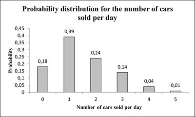
Example: Probability distribution for the number of cars sold per day at a dealership:

x	f(x)
0	0.18
1	0.39
2	0.24
3	0.14
4	0.04
5	0.01

Calculating Probabilities

• Probability of exactly 2 cars sold: $P(X = 2) = 0.24$

• Probability of at most 2 cars sold: $P(X \leq 2) = f(0) + f(1) + f(2) = 0.81$

• Probability of more than 2 cars sold: $P(X > 2) = f(3) + f(4) + f(5) = 0.19$

• Probability of at least 2 cars sold: $P(X \geq 2) = f(2) + f(3) + f(4) + f(5) = 0.43$

• Probability of more than 1 but less than 4 cars sold: $P(1 < X < 4) = f(2) + f(3) = 0.38$

Discrete Uniform Probability Distribution

A discrete random variable has a uniform distribution if all possible values are equally likely. The PMF is:

$f(x) = \frac{1}{n}$ for $x = x_1, x_2, ..., x_n$

Example: Rolling a fair die ($n = 6$): $f(x) = \frac{1}{6}$ for $x = 1, 2, 3, 4, 5, 6$.

Expected Value and Variance

Definitions and Formulas

• Expected Value (Mean): $E(X) = \mu = \sum x f(x)$

• Variance: $Var(X) = \sigma^2 = \sum (x - \mu)^2 f(x)$

• Standard Deviation: $\sigma = \sqrt{\sigma^2}$

Example: For the car sales distribution above:

• $E(X) = 1.5$

• $Var(X) = 1.25$

• $\sigma = 1.118$

The Binomial Distribution

Definition and Properties

The binomial distribution models the number of successes in a fixed number of independent trials, each with the same probability of success.

• Properties:

  1. n identical trials

  2. Each trial has two outcomes: success or failure

  3. Probability of success (p) is constant

  4. Trials are independent

Probability Mass Function:

$f(x) = \binom{n}{x} p^x (1-p)^{n-x}$

where $x = 0, 1, ..., n$

Expected Value and Variance:

$E(X) = np$

$Var(X) = np(1-p)$

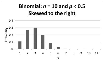
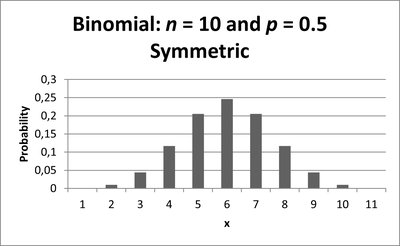
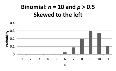
Shape of the Binomial Distribution

• If $p = 0.5$, the distribution is symmetric.

• If $p < 0.5$, it is skewed to the right.

• If $p > 0.5$, it is skewed to the left.

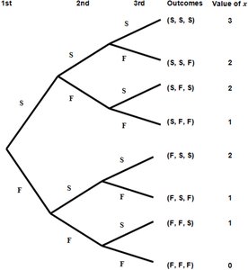
Example: Binomial Experiment with n = 3, p = 0.3

• Let X = number of customers making a purchase out of 3.

• Tree diagram illustrates all possible outcomes and values of X.

• $P(X = 2) = 0.189$

• $P(X = 1) = 0.441$

• $P(X = 3) = 0.027$

• $P(X = 0) = 0.343$

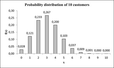
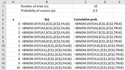
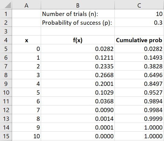
Example: Binomial Distribution for n = 10, p = 0.3

• $E(X) = 3$

• $Var(X) = 2.1$

• $\sigma = 1.449$

Using Excel for Binomial Probabilities

Excel functions such as BINOM.DIST can be used to compute binomial probabilities and cumulative probabilities.

Common Probability Calculations with the Binomial Distribution

• At most k successes: $P(X \leq k)$ (sum of probabilities up to k)

• Exactly k successes: $P(X = k)$

• More than k successes: $P(X > k) = 1 - P(X \leq k)$

• Between a and b successes: $P(a < X < b) = P(X \leq b-1) - P(X \leq a)$

Continuous Probability Distributions (Preview)

Continuous Random Variables and Probability Density Function (PDF)

• Continuous Random Variable: Can take any value within an interval.

• Probability Density Function (PDF): $f(x)$, where $P(a \leq X \leq b) = \int_a^b f(x) dx$

• Properties of a PDF:

  • $f(x) \geq 0$ for all x

  • $\int_{-\infty}^{\infty} f(x) dx = 1$

Additional info: The chapter continues with continuous distributions, but the main focus here is on discrete probability distributions and the binomial distribution.