Discrete Probability Distributions: Discrete, Binomial, Poisson, and Hypergeometric Distributions

Discrete Probability Distributions

Discrete Random Variables

Discrete random variables (DRVs) are variables that can take on a countable number of distinct values. They are fundamental in probability and statistics for modeling outcomes of experiments where results are countable and not continuous.

• Definition: A random variable assigns a single numerical value to each outcome of a random experiment.

• Discrete Random Variable (DRV): Values cannot be broken down further (e.g., number of defective bulbs, dice rolls).

• Continuous Random Variable (CRV): Values can be broken down further (e.g., height, time).

• Probability Distribution: A table or function that shows the probabilities of all possible values a random variable can take.

Example: The number of defective lightbulbs in a batch, or the number of sodas consumed per day, are discrete random variables.

Probability Distribution Criteria

• Each probability must be between 0 and 1, inclusive.

• The sum of all probabilities must equal 1.

Example Table: (Lottery Profits)

Profit	Probability
-$1.00	0.40
$0.00	0.35
$5.00	?
$1,000,000.00	0.01

To find the missing probability, ensure the sum is 1.

Identifying Discrete Random Variables

• Countable outcomes (e.g., number of defective bulbs, number of days in a month) are discrete.

• Measurements (e.g., time, weight) are continuous.

Calculating Probabilities from Distributions

To find the probability of a range of outcomes, sum the probabilities for the relevant values.

Example Table: (Sodas per Day)

Sodas per Day	Probability
0	0.50
1	0.31
2	0.09
3	0.05
4	0.03
5	0.01
6	0.01

Example: Probability of at most 2 sodas per day = 0.50 + 0.31 + 0.09 = 0.90.

Mean (Expected Value), Variance, and Standard Deviation of DRVs

Expected Value (Mean)

The expected value (mean) of a discrete random variable is the long-run average value of repetitions of the experiment it represents.

• Formula: $\mu = \sum x \cdot P(x)$

• Multiply each value by its probability, then sum the results.

Example Table: (Number of Kids per Household)

# of Kids	Probability
0	0.15
1	0.60
2	0.25

Expected Value: $\mu = 0 \times 0.15 + 1 \times 0.60 + 2 \times 0.25 = 1.10$

Variance and Standard Deviation

• Variance: $\sigma^2 = \sum (x - \mu)^2 P(x)$

• Standard Deviation: $\sigma = \sqrt{\sigma^2}$

Example: For the above table, calculate each $(x - \mu)^2 P(x)$ and sum for variance.

Binomial Distribution

Definition and Properties

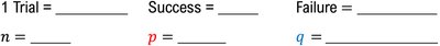
The binomial distribution models the number of successes in a fixed number of independent trials, each with the same probability of success.

• Each trial has two outcomes: success or failure.

• There are a fixed number of trials ($n$).

• Trials are independent.

• Probability of success ($p$) is constant for each trial.

Binomial Probability Formula

• Probability of exactly $k$ successes in $n$ trials:

$P(X = k) = \binom{n}{k} p^k q^{n-k}$

• $\binom{n}{k}$ is the number of combinations of $n$ items taken $k$ at a time.

• $p$ is the probability of success, $q = 1 - p$ is the probability of failure.

Mean and Standard Deviation of Binomial Distribution

• Mean: $\mu = np$

• Variance: $\sigma^2 = npq$

• Standard Deviation: $\sigma = \sqrt{npq}$

Finding Binomial Probabilities with Technology

Use calculators or statistical software for large $n$ or cumulative probabilities.

• binompdf: For exact probabilities.

• binomcdf: For cumulative probabilities (e.g., "at most", "at least").

Poisson Distribution

Definition and Properties

The Poisson distribution models the number of occurrences of an event in a fixed interval of time or space, given the average rate of occurrence ($\lambda$).

• Events occur independently.

• The mean number of occurrences in the interval is $\lambda$.

Poisson Probability Formula:

$P(X = x) = \frac{\lambda^x e^{-\lambda}}{x!}$

• Mean: $\mu = \lambda$

• Variance: $\sigma^2 = \lambda$

When to Use Poisson vs. Binomial

• Use Poisson when counting occurrences in a fixed interval and $n$ is large, $p$ is small.

• Use Binomial for a fixed number of independent trials with two outcomes.

Finding Poisson Probabilities with Technology

• poissonpdf: For exact probabilities.

• poissoncdf: For cumulative probabilities.

Hypergeometric Distribution

Definition and Properties

The hypergeometric distribution models the probability of $x$ successes in $n$ draws from a finite population of size $N$ containing $r$ successes, without replacement.

• Trials are not independent (no replacement).

• Probability of success changes on each draw.

Hypergeometric Probability Formula:

$P(X = x) = \frac{\binom{r}{x} \binom{N - r}{n - x}}{\binom{N}{n}}$

Comparison Table: Binomial vs. Hypergeometric

Property	Binomial	Hypergeometric
Replacement	With replacement (independent)	Without replacement (dependent)
Probability of Success	Constant	Changes each draw
Population Size	Usually large or infinite	Finite

Summary Table: Key Formulas

Distribution	Mean ($\mu$)	Variance ($\sigma^2$)	Probability Formula
Discrete RV	$\sum x P(x)$	$\sum (x - \mu)^2 P(x)$	Given by table
Binomial	$np$	$npq$	$\binom{n}{k} p^k q^{n-k}$
Poisson	$\lambda$	$\lambda$	$\frac{\lambda^x e^{-\lambda}}{x!}$
Hypergeometric	---	---	$\frac{\binom{r}{x} \binom{N - r}{n - x}}{\binom{N}{n}}$

Additional info: For all distributions, technology (such as the TI-84 calculator) can be used to compute probabilities efficiently, especially for cumulative probabilities or large sample sizes.