Discrete Probability Distributions: Study Guide for Statistics Students

Discrete Probability Distributions

Discrete Random Variables

Discrete random variables (DRVs) are fundamental in statistics, representing outcomes that can only take specific, countable values. Understanding the distinction between discrete and continuous random variables is essential for analyzing probability distributions.

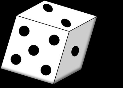
• Discrete Random Variable (DRV): A variable whose possible values are countable and cannot be broken down further (e.g., number of defective lightbulbs).

• Continuous Random Variable (CRV): A variable whose possible values form an interval and can be broken down infinitely (e.g., height, time).

• Probability Distribution: A table or function that shows the probabilities of all possible values a random variable can take.

• Example: The number of sodas consumed per day, or the number of prizes won in a raffle.

Probability Distribution Tables

Probability distributions for DRVs are often represented in tables, which must satisfy two criteria:

• All probabilities must be between 0 and 1.

• The sum of all probabilities must equal 1.

Example Table: Lottery Profits

Profit	Probability
-$1.00	0.40
$0.00	0.35
$5.00	?
$1,000,000.00	0.01

Additional info: The missing probability can be found by subtracting the sum of the known probabilities from 1.

Mean (Expected Value) of a Discrete Random Variable

The mean or expected value of a DRV is the long-run average value of the variable, calculated by multiplying each value by its probability and summing the results.

• Formula: $\mu = \sum [x \cdot P(x)]$

• Example: Number of kids per household.

# of Kids	Probability
0	0.15
1	0.60
2	0.25

Variance and Standard Deviation of Discrete Random Variables

Variance and standard deviation measure the spread of a probability distribution. They are calculated using the mean and the probabilities of each outcome.

• Variance Formula: $\sigma^2 = \sum [(x - \mu)^2 \cdot P(x)]$

• Standard Deviation Formula: $\sigma = \sqrt{\sigma^2}$

Example Table: Number of complaints received daily.

# of Complaints	Probability
0	0.45
1	0.30
2	0.20
3	0.05

Binomial Distribution

The Binomial Experiment

The binomial distribution models the number of successes in a fixed number of independent trials, each with the same probability of success. It is widely used for scenarios with two possible outcomes (success or failure).

• Criteria: Fixed number of trials, only two outcomes per trial, independent trials, constant probability of success.

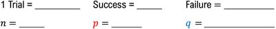
• Parameters: $n$ = number of trials, $p$ = probability of success, $q$ = probability of failure ($q = 1 - p$).

Binomial Probability Formula

To find the probability of exactly $k$ successes in $n$ trials:

• Formula: $P(X = k) = \binom{n}{k} p^k q^{n-k}$

• Example: Probability of getting exactly 3 red marbles in 4 draws, with replacement.

Mean and Standard Deviation of Binomial Distribution

The mean and standard deviation of a binomial distribution can be calculated directly from its parameters:

• Mean: $\mu = n p$

• Standard Deviation: $\sigma = \sqrt{n p q}$

Finding Binomial Probabilities Using TI-84 Calculator

Binomial probabilities can be calculated using the TI-84 calculator functions:

• binompdf: For exact probabilities.

• binomcdf: For cumulative probabilities (e.g., "at most", "at least").

Poisson Distribution

Intro to Poisson Distribution

The Poisson distribution models the number of occurrences of an event in a fixed interval of time or space, given a known average rate. It is used when events occur independently and the probability of more than one event in a small interval is negligible.

• Parameter: $\lambda$ = mean number of events in the interval.

• Formula: $P(x) = \frac{\lambda^x e^{-\lambda}}{x!}$

• Mean and Variance: $\mu = \lambda$, $\sigma^2 = \lambda$

Finding Poisson Probabilities Using TI-84 Calculator

Poisson probabilities can be calculated using the TI-84 calculator functions:

• poissonpdf: For exact probabilities.

• poissoncdf: For cumulative probabilities.

Using Poisson to Approximate Binomial Probabilities

When the number of trials is large and the probability of success is small, the Poisson distribution can approximate the binomial distribution:

• Approximation: $\lambda = n p$

• Requirements: $n \geq 100$, $p \leq 0.01$

Hypergeometric Distribution

Intro to Hypergeometric Distribution

The hypergeometric distribution models the probability of $x$ successes in $n$ draws from a finite population of $N$ items, without replacement. It differs from the binomial distribution in that the probability of success changes with each draw.

• Parameters: $N$ = population size, $r$ = number of successes in population, $n$ = number of draws.

• Formula: $P(x) = \frac{\binom{r}{x} \binom{N - r}{n - x}}{\binom{N}{n}}$

Comparison Table: Binomial vs. Hypergeometric Distribution

Distribution	Replacement	Probability of Success
Binomial	With replacement	Constant
Hypergeometric	Without replacement	Changes with each draw

Additional info: Hypergeometric distribution is used when sampling without replacement from a finite population.