Discrete Probability Distributions: Study Guide for Statistics Students

Discrete Probability Distributions

Discrete and Continuous Random Variables

Random variables are numerical measures of outcomes from probability experiments, determined by chance. They are denoted by letters such as X. There are two main types:

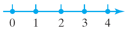
• Discrete Random Variable: Has a finite or countable number of values. These values can be plotted on a number line with space between each point.

• Continuous Random Variable: Has infinitely many values, which can be plotted on a line in an uninterrupted fashion.

Examples:

• The number of light bulbs that burn out in a room of 10 light bulbs in the next year: Discrete; possible values: 0, 1, ..., 10

• The number of leaves on a randomly selected oak tree: Discrete; possible values: 0, 1, 2, ...

• The length of time between calls to 911: Continuous; possible values: t > 0

Discrete Probability Distributions

A probability distribution provides the possible values of the random variable X and their corresponding probabilities. It can be represented as a table, graph, or mathematical formula.

Rules for a Discrete Probability Distribution:

• The sum of all probabilities must equal 1: $\sum P(x) = 1$

• Each probability must be between 0 and 1: $0 \leq P(x) \leq 1$

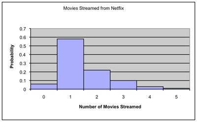
Example Table: Probability distribution for the number of movies streamed on Netflix each month:

x	P(x)
0	0.06
1	0.58
2	0.22
3	0.10
4	0.03
5	0.01

Probability Histograms

A probability histogram is a graphical representation where the horizontal axis corresponds to the value of the random variable and the vertical axis represents the probability of that value.

Mean of a Discrete Random Variable

The mean (or expected value) of a discrete random variable is calculated as:

$\mu_X = \sum x \cdot P(x)$

Where x is the value of the random variable and P(x) is the probability of observing that value.

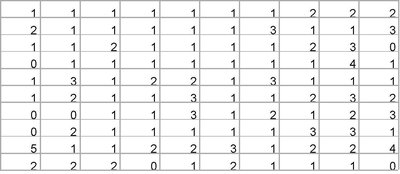
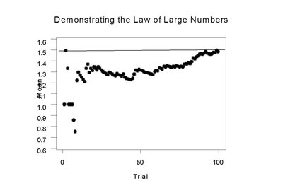
Example Calculation:

• $\mu_X = 0 \cdot 0.06 + 1 \cdot 0.58 + 2 \cdot 0.22 + 3 \cdot 0.10 + 4 \cdot 0.03 + 5 \cdot 0.01 = 1.49$

Interpretation: As the number of repetitions of the experiment increases, the mean value of the trials will approach $\mu_X$. This demonstrates the Law of Large Numbers.

Expected Value

The mean of a random variable represents what we would expect to happen in the long run and is also called the expected value, denoted as E(X).

Standard Deviation of a Discrete Random Variable

The standard deviation measures the spread of the values of a discrete random variable. It is calculated as:

$\sigma_X = \sqrt{\sum (x - \mu_X)^2 \cdot P(x)}$

Alternatively, the variance is:

$\sigma_X^2 = \sum x^2 \cdot P(x) - \mu_X^2$

Example Calculation: For the DVD rental distribution, the variance and standard deviation are computed stepwise for each value of x.

Binomial Probability Distribution

Criteria for a Binomial Probability Experiment

An experiment is a binomial experiment if:

• It is performed a fixed number of times (trials).

• Trials are independent.

• Each trial has two mutually exclusive outcomes: success or failure.

• The probability of success is fixed for each trial.

Notation

• n: Number of independent trials

• p: Probability of success

• X: Binomial random variable (number of successes in n trials)

Binomial Probability Distribution Function

The probability of obtaining x successes in n independent trials is:

$P(x) = \binom{n}{x} p^x (1-p)^{n-x}$

Where $\binom{n}{x}$ is the binomial coefficient.

Mean and Standard Deviation of a Binomial Random Variable

For a binomial experiment:

• Mean: $\mu_X = n p$

• Standard deviation: $\sigma_X = \sqrt{n p (1-p)}$

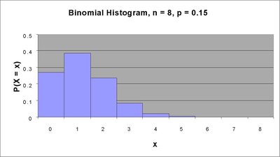
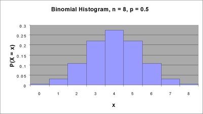
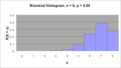
Binomial Probability Histograms

Binomial probability histograms visually represent the distribution of the number of successes for given n and p values. The shape of the distribution changes with p:

• For small p, the distribution is skewed right.

• For p = 0.5, the distribution is symmetric.

• For large p, the distribution is skewed left.

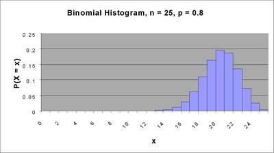
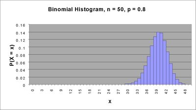
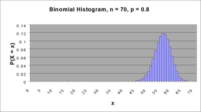
As n increases, the distribution becomes bell-shaped. If $n p (1-p) > 10$, the distribution is approximately normal.

Empirical Rule for Binomial Experiments

The Empirical Rule states that in a bell-shaped distribution, about 95% of all observations lie within two standard deviations of the mean:

$\mu_X - 2\sigma_X$ to $\mu_X + 2\sigma_X$

Observations outside this interval are considered unusual.

Poisson Probability Distribution

Criteria for a Poisson Process

A random variable X follows a Poisson process if:

• The probability of two or more successes in any sufficiently small subinterval is 0.

• The probability of success is the same for any two intervals of equal length.

• The number of successes in any interval is independent of the number in any other non-overlapping interval.

Poisson Probability Distribution Function

If X is the number of successes in an interval of fixed length t, the probability of obtaining x successes is:

$P(x) = \frac{(\lambda t)^x}{x!} e^{-\lambda t}$

Where $\lambda$ is the average number of occurrences per interval of length 1, and $e \approx 2.71828$.

Mean and Standard Deviation of a Poisson Random Variable

For a Poisson process with parameter $\lambda$:

• Mean: $\mu_X = \lambda t$

• Standard deviation: $\sigma_X = \sqrt{\lambda t}$

Example: If $\lambda = 0.6$ insect fragments per gram, in a 5-gram sample:

• Mean: $\mu_X = 0.6 \times 5 = 3$

• Standard deviation: $\sigma_X = \sqrt{3} \approx 1.73$